interp1
1-D data interpolation (table lookup)
Syntax
Description
vq = interp1(x,v,xq)interp1 uses linear interpolation. Vector
x contains the sample points, and v
contains the corresponding values, v(x).
Vector xq contains the coordinates of the query
points.
If you have multiple sets of data that are sampled at the same point
coordinates, then you can pass v as an array. Each column of
array v contains a different set of 1-D sample values.
vq = interp1(x,v,xq,method,extrapolation)x. Set extrapolation to
'extrap' when you want to use the
method algorithm for extrapolation. Alternatively, you
can specify a scalar value, in which case, interp1 returns
that value for all points outside the domain of x.
vq = interp1(v,xq)1 to n, where n
depends on the shape of v:
When v is a vector, the default points are
1:length(v).When v is an array, the default points are
1:size(v,1).
Use this syntax when you are not concerned about the absolute distances between points.
vq = interp1(v,xq,method,extrapolation)
pp = interp1(x,v,method,'pp')method algorithm.
Note
This syntax is not recommended. Use griddedInterpolant
instead.
Examples
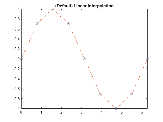
Interpolation of Coarsely Sampled Sine Function
Define the sample points, x, and corresponding sample values, v.
x = 0:pi/4:2*pi;
v = sin(x);
Define the query points to be a finer sampling over the range of x.
xq = 0:pi/16:2*pi;
Interpolate the function at the query points and plot the result.
figure
vq1 = interp1(x,v,xq);
plot(x,v,'o',xq,vq1,':.');
xlim([0 2*pi]);
title('(Default) Linear Interpolation');
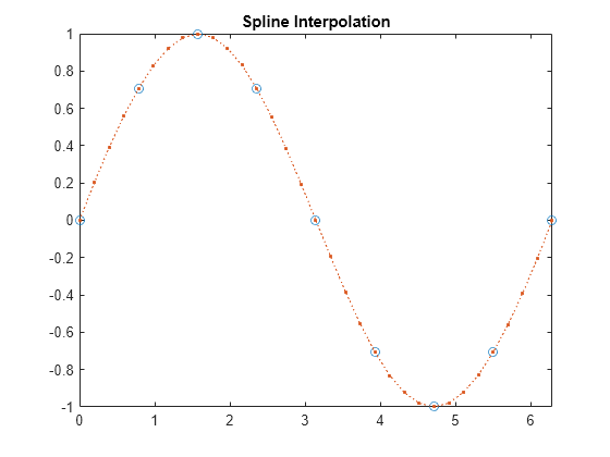
Now evaluate v at the same points using the 'spline' method.
figure
vq2 = interp1(x,v,xq,'spline');
plot(x,v,'o',xq,vq2,':.');
xlim([0 2*pi]);
title('Spline Interpolation');
Interpolation Without Specifying Points
Define a set of function values.
v = [0 1.41 2 1.41 0 -1.41 -2 -1.41 0];
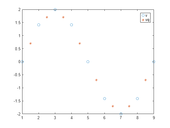
Define a set of query points that fall between the default points, 1:9. In this case, the default points are 1:9 because v contains 9 values.
xq = 1.5:8.5;
Evaluate v at xq.
vq = interp1(v,xq);
Plot the result.
figure
plot((1:9),v,'o',xq,vq,'*');
legend('v','vq');
Interpolation of Complex Values
Define a set of sample points.
x = 1:10;
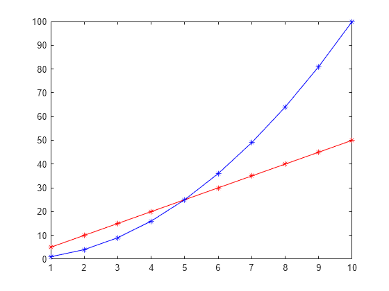
Define the values of the function, , at the sample points.
v = (5*x)+(x.^2*1i);
Define the query points to be a finer sampling over the range of x.
xq = 1:0.25:10;
Interpolate v at the query points.
vq = interp1(x,v,xq);
Plot the real part of the result in red and the imaginary part in blue.
figure
plot(x,real(v),'*r',xq,real(vq),'-r');
hold on
plot(x,imag(v),'*b',xq,imag(vq),'-b');
Interpolation of Dates and Times
Interpolate time-stamped data points.
Consider a data set containing temperature readings that are measured every four hours. Create a table with one day's worth of data and plot the data.
x = (datetime(2016,1,1):hours(4):datetime(2016,1,2))';
x.Format = 'MMM dd, HH:mm';
T = [31 25 24 41 43 33 31]';
WeatherData = table(x,T,'VariableNames',{'Time','Temperature'})
WeatherData=7×2 table
        Time         Temperature
    _____________    ___________

    Jan 01, 00:00        31
    Jan 01, 04:00        25
    Jan 01, 08:00        24
    Jan 01, 12:00        41
    Jan 01, 16:00        43
    Jan 01, 20:00        33
    Jan 02, 00:00        31
plot(WeatherData.Time, WeatherData.Temperature, 'o')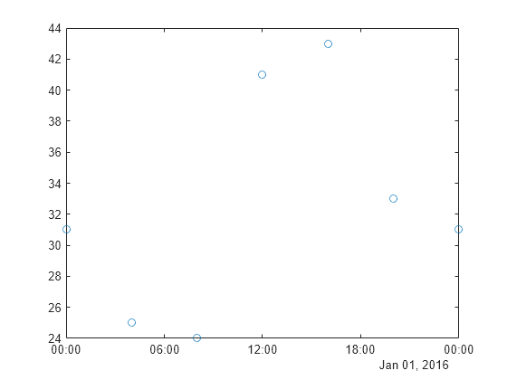
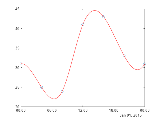
Interpolate the data set to predict the temperature reading during each minute of the day. Since the data is periodic, use the 'spline' interpolation method.
xq = (datetime(2016,1,1):minutes(1):datetime(2016,1,2))';
V = interp1(WeatherData.Time, WeatherData.Temperature, xq, 'spline');
Plot the interpolated points.
hold on
plot(xq,V,'r')
Extrapolation Using Two Different Methods
Define the sample points, x, and corresponding sample values, v.
x = [1 2 3 4 5];
v = [12 16 31 10 6];
Specify the query points, xq, that extend beyond the domain of x.
xq = [0 0.5 1.5 5.5 6];
Evaluate v at xq using the 'pchip' method.
vq1 = interp1(x,v,xq,'pchip')vq1 = 1×5
19.3684 13.6316 13.2105 7.4800 12.5600
Next, evaluate v at xq using the 'linear' method.
vq2 = interp1(x,v,xq,'linear')vq2 = 1×5
NaN NaN 14 NaN NaN
Now, use the 'linear' method with the 'extrap' option.
vq3 = interp1(x,v,xq,'linear','extrap')
vq3 = 1×5

     8    10    14     4     2
'pchip' extrapolates by default, but 'linear' does not.
Designate Constant Value for All Queries Outside the Domain of x
Define the sample points, x, and corresponding sample values, v.
x = [-3 -2 -1 0 1 2 3];
v = 3*x.^2;
Specify the query points, xq, that extend beyond the domain of x.
xq = [-4 -2.5 -0.5 0.5 2.5 4];
Now evaluate v at xq using the 'pchip' method and assign any values outside the domain of x to the value, 27.
vq = interp1(x,v,xq,'pchip',27)vq = 1×6
27.0000 18.6562 0.9375 0.9375 18.6562 27.0000
Interpolate Multiple Sets of Data in One Pass
Define the sample points.
x = (-5:5)';
Sample three different parabolic functions at the points defined in x.
v1 = x.^2;
v2 = 2*x.^2 + 2;
v3 = 3*x.^2 + 4;
Create matrix v, whose columns are the vectors, v1, v2, and v3.
v = [v1 v2 v3];
Define a set of query points, xq, to be a finer sampling over the range of x.
xq = -5:0.1:5;
Evaluate all three functions at xq and plot the results.
vq = interp1(x,v,xq,'pchip');
figure
plot(x,v,'o',xq,vq);

h = gca;
h.XTick = -5:5;
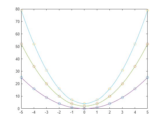
The circles in the plot represent v, and the solid lines represent vq.
Input Arguments
x — Sample points
vector
Sample points, specified as a row or column vector of real numbers. The
values in x must be distinct. The length of
x must conform to one of the following requirements:
If
vis a vector, thenlength(x)must equallength(v).If
vis an array, thenlength(x)must equalsize(v,1).
Example: [1 2 3 4 5 6 7 8 9 10]
Example: 1:10
Example: [3 7 11 15 19 23 27 31]'
Data Types: single | double | duration | datetime
v — Sample values
vector | matrix | array
Sample values, specified as a vector, matrix, or array of real or complex
numbers. If v is a matrix or an array, then each column
contains a separate set of 1-D values.
If v contains complex numbers, then
interp1 interpolates the real and imaginary parts
separately.
Example: rand(1,10)
Example: rand(10,1)
Example: rand(10,3)
Data Types: single | double | duration | datetime
Complex Number Support: Yes
xq — Query points
scalar | vector | matrix | array
Query points, specified as a scalar, vector, matrix, or array of real numbers.
Example: 5
Example: 1:0.05:10
Example: (1:0.05:10)'
Example: [0 1 2 7.5 10]
Data Types: single | double | duration | datetime
method — Interpolation method
'linear' (default) | 'nearest' | 'next' | 'previous' | 'pchip' | 'cubic' | 'v5cubic' | 'makima' | 'spline'
Interpolation method, specified as one of the options in this table.
Method | Description | Continuity | Comments |
|---|---|---|---|
| Linear interpolation. The interpolated value at a query point is based on linear interpolation of the values at neighboring grid points in each respective dimension. This is the default interpolation method. | C0 |
|
| Nearest neighbor interpolation. The interpolated value at a query point is the value at the nearest sample grid point. | Discontinuous |
|
| Next neighbor interpolation. The interpolated value at a query point is the value at the next sample grid point. | Discontinuous |
|
| Previous neighbor interpolation. The interpolated value at a query point is the value at the previous sample grid point. | Discontinuous |
|
| Shape-preserving piecewise cubic interpolation. The interpolated value at a query point is based on a shape-preserving piecewise cubic interpolation of the values at neighboring grid points. | C1 |
|
| Cubic convolution used in MATLAB® 5. | C1 |
|
| Same as
| C1 | |
| Modified Akima cubic Hermite interpolation. The interpolated value at a query point is based on a piecewise function of polynomials with degree at most three. The Akima formula is modified to avoid overshoots. | C1 |
|
| Spline interpolation using not-a-knot end conditions. The interpolated value at a query point is based on a cubic interpolation of the values at neighboring grid points in each respective dimension. | C2 |
|
extrapolation — Extrapolation strategy
'extrap' | scalar value
Extrapolation strategy, specified as 'extrap' or a real
scalar value.
Specify
'extrap'when you wantinterp1to evaluate points outside the domain using the same method it uses for interpolation.Specify a scalar value when you want
interp1to return a specific constant value for points outside the domain.
The default behavior depends on the input arguments:
If you specify the
'pchip','spline', or'makima'interpolation methods, then the default behavior is'extrap'.All other interpolation methods return
NaNby default for query points outside the domain.
Example: 'extrap'
Example: 5
Data Types: char | string | single | double
Output Arguments
vq — Interpolated values
scalar | vector | matrix | array
Interpolated values, returned as a scalar, vector, matrix, or array. The
size of vq depends on the shape of v
and xq.
| Shape of v | Shape of xq | Size of Vq | Example |
|---|---|---|---|
| Vector | Vector | size(xq) | If size(v) = [1
100]and size(xq) =
[1 500], then size(vq) = [1 500]. |
| Vector | Matrix or N-D Array | size(xq) | If size(v) = [1
100]and size(xq) =
[50 30], then size(vq) = [50 30]. |
| Matrix or N-D Array | Vector | [length(xq)
size(v,2),...,size(v,n)] | If size(v) = [100
3]and size(xq) = [1
500], then size(vq) = [500 3]. |
| Matrix or N-D Array | Matrix or N-D Array | [size(xq,1),...,size(xq,n),...
size(v,2),...,size(v,m)] | If size(v) = [4 5
6]and size(xq) = [2
3 7], then size(vq) = [2 3 7 5 6]. |
pp — Piecewise polynomial
structure
Piecewise polynomial, returned as a structure that you can pass to the
ppval function for
evaluation.
More About
Akima and Spline Interpolation
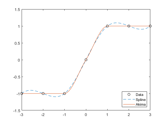
The Akima algorithm for one-dimensional interpolation, described in [1] and [2], performs cubic interpolation to produce piecewise polynomials with continuous first-order derivatives (C1). The algorithm preserves the slope and avoids undulations in flat regions. A flat region occurs whenever there are three or more consecutive collinear points, which the algorithm connects with a straight line. To ensure that the region between two data points is flat, insert an additional data point between those two points.
When two flat regions with different slopes meet, the modification made to the original Akima algorithm gives more weight to the side where the slope is closer to zero. This modification gives priority to the side that is closer to horizontal, which is more intuitive and avoids the overshoot. (The original Akima algorithm gives equal weights to the points on both sides, thus evenly dividing the undulation.)
The spline algorithm, on the other hand, performs cubic interpolation to produce piecewise polynomials with continuous second-order derivatives (C2). The result is comparable to a regular polynomial interpolation, but is less susceptible to heavy oscillation between data points for high degrees. Still, this method can be susceptible to overshoots and oscillations between data points.
Compared to the spline algorithm, the Akima algorithm produces fewer undulations and is better suited to deal with quick changes between flat regions. This difference is illustrated below using test data that connects multiple flat regions.
References
[1] Akima, Hiroshi. "A new method of interpolation and smooth curve fitting based on local procedures." Journal of the ACM (JACM) , 17.4, 1970, pp. 589-602.
[2] Akima, Hiroshi. "A method of bivariate interpolation and smooth surface fitting based on local procedures." Communications of the ACM , 17.1, 1974, pp. 18-20.
Extended Capabilities
C/C++ Code Generation
Generate C and C++ code using MATLAB® Coder™.
Usage notes and limitations:
The input argument
x(sample points) must be strictly increasing or strictly decreasing. Indices are not reordered.If the input argument
v(sample values) is a variable-length vector (1-by-:or:-by-1), then the shape of the outputvqmatches the shape in MATLAB.If the input argument
vis variable-size, is not a variable-length vector, and becomes a row vector at run time, then an error occurs.If the sample values or query points contain
Infor-Inf, the output of the generated code might not match the output in MATLAB.If the input argument
xq(query points) is variable-size, is not a variable-length vector, and becomes a row or column vector at run time, then an error occurs.See Variable-Sizing Restrictions for Code Generation of Toolbox Functions (MATLAB Coder).
GPU Code Generation
Generate CUDA® code for NVIDIA® GPUs using GPU Coder™.
Usage notes and limitations:
The input argument
x(sample points) must be strictly increasing or strictly decreasing. Indices are not reordered.If the input argument
v(sample values) is a variable-length vector (1-by-:or:-by-1), then the shape of the outputvqmatches the shape in MATLAB.If the input argument
vis variable-size, is not a variable-length vector, and becomes a row vector at run time, then an error occurs.If the input argument
xq(query points) is variable-size, is not a variable-length vector, and becomes a row or column vector at run time, then an error occurs.See Variable-Sizing Restrictions for Code Generation of Toolbox Functions (MATLAB Coder).
Thread-Based Environment
Run code in the background using MATLAB® backgroundPool or accelerate code with Parallel Computing Toolbox™ ThreadPool.
This function fully supports thread-based environments. For more information, see Run MATLAB Functions in Thread-Based Environment.
GPU Arrays
Accelerate code by running on a graphics processing unit (GPU) using Parallel Computing Toolbox™.
The interp1 function
supports GPU array input with these usage notes and limitations:
The interpolation methods
'pchip'and'makima'are not supported.The
'spline'interpolation method is not supported for sample valuesvcontainingNaN.
For more information, see Run MATLAB Functions on a GPU (Parallel Computing Toolbox).
Distributed Arrays
Partition large arrays across the combined memory of your cluster using Parallel Computing Toolbox™.
This function fully supports distributed arrays. For more information, see Run MATLAB Functions with Distributed Arrays (Parallel Computing Toolbox).
Version History
Introduced before R2006aR2020b: 'cubic' method of interp1 performs cubic convolution
In R2020b, the 'cubic' interpolation method of
interp1 performs cubic convolution. The
'v5cubic' and 'cubic' interpolation
methods now perform the same type of interpolation, which is consistent with the
behavior of interp2, interp3, and
interpn. The cubic convolution interpolation method is
intended for uniformly-spaced data, and it falls back to 'spline'
interpolation for irregularly-spaced data.
In previous releases, 'cubic' was the same as
'pchip', and only 'v5cubic' performed
cubic convolution.
See Also
MATLAB Command
You clicked a link that corresponds to this MATLAB command:
Run the command by entering it in the MATLAB Command Window. Web browsers do not support MATLAB commands.

Select a Web Site
Choose a web site to get translated content where available and see local events and offers. Based on your location, we recommend that you select: .
You can also select a web site from the following list
How to Get Best Site Performance
Select the China site (in Chinese or English) for best site performance. Other bat365 country sites are not optimized for visits from your location.
Americas
- América Latina (Español)
- Canada (English)
- United States (English)
Europe
- Belgium (English)
- Denmark (English)
- Deutschland (Deutsch)
- España (Español)
- Finland (English)
- France (Français)
- Ireland (English)
- Italia (Italiano)
- Luxembourg (English)
- Netherlands (English)
- Norway (English)
- Österreich (Deutsch)
- Portugal (English)
- Sweden (English)
- Switzerland
- United Kingdom (English)
Asia Pacific
- Australia (English)
- India (English)
- New Zealand (English)
- 中国
- 日本Japanese (日本語)
- 한국Korean (한국어)