figure
Create figure window
Description
figure creates a new figure window using
default property values. The resulting figure is the current figure.
figure( modifies
properties of the figure using one or more name-value pair arguments.
For example, Name,Value)figure('Color','white') sets the background
color to white.
figure( makes the
figure specified by f)f the current figure and
displays it on top of all other figures.
figure( finds a
figure in which the n)Number property is equal
to n, and makes it the current figure. If no
figure exists with that property value, MATLAB® creates a new
figure and sets its Number property to n.
Examples
Change Figure Size
Create a default figure.
f = figure;
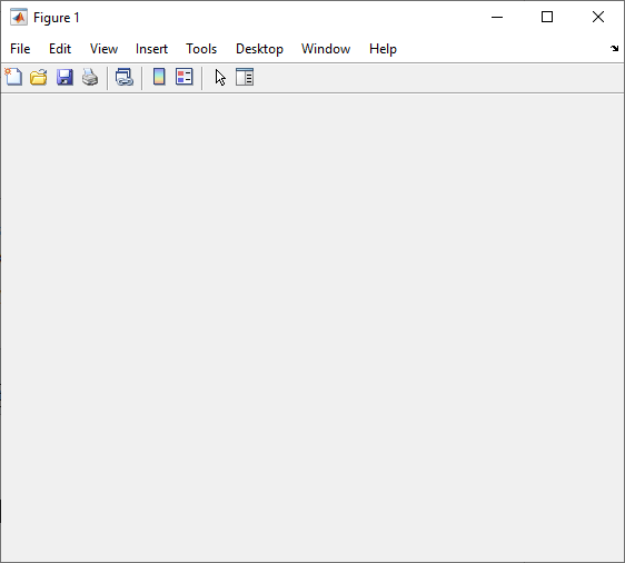
Get the location, width, and height of the figure.
f.Position
ans =

   680   558   560   420
This means that the figure window is positioned 680 pixels to the right and 558 pixels above the bottom left corner of the primary display, and is 560 pixels wide and 420 pixels tall.
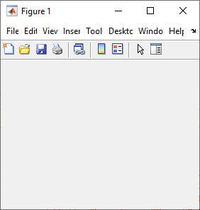
Halve the figure width and height by adjusting the third and fourth elements of the position vector.
f.Position(3:4) = [280 210];
Specify Figure Title
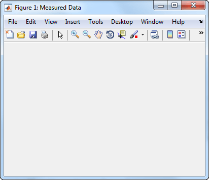
Create a figure, and specify the Name property.
By default, the resulting title includes the figure number.
figure('Name','Measured Data');
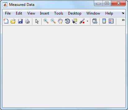
Specify the Name property again,
but this time, set the NumberTitle property to 'off'.
The resulting title does not include the figure number.
figure('Name','Measured Data','NumberTitle','off');
Working with Multiple Figures Simultaneously
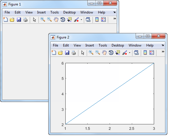
Create two figures, and then create a line plot. By default,
the plot command targets the current figure.
f1 = figure;
f2 = figure;
plot([1 2 3],[2 4 6]);
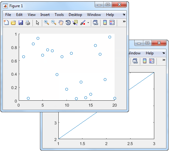
Set the current figure to f1, so that
it is the target for the next plot. Then create a scatter plot.
figure(f1);
scatter((1:20),rand(1,20));
Input Arguments
f — Target figure
Figure object
Target figure, specified as a Figure object.
n — Target figure number
scalar integer value
Target figure number, specified as a scalar integer value. When you specify this argument,
MATLAB searches for an existing figure in which the Number property is
equal to n. If no figure exists with that property value,
MATLAB creates a new figure and sets its Number
property to n. By default, the
Number property value is displayed in the title of
the figure.
Data Types: double
Name-Value Arguments
Specify optional pairs of arguments as
Name1=Value1,...,NameN=ValueN, where Name is
the argument name and Value is the corresponding value.
Name-value arguments must appear after other arguments, but the order of the
pairs does not matter.
Example: figure(Color="white") creates a figure with a white
background.
Before R2021a, use commas to separate each name and value, and enclose
Name in quotes.
Example: figure("Color","white") creates a figure with a white
background.
Note
The properties listed here are only a subset. For a full list, see Figure Properties.
Name — Name
'' (default) | character vector | string scalar
Name of the figure, specified as a character vector or a string scalar.
Example: figure('Name','Results') sets the name of the figure to
'Results'.
By default, the name is 'Figure n', where
n is an integer. When you specify the
Name property, the title of the figure becomes 'Figure
n: name'. If you want only
the Name value to appear, set IntegerHandle or
NumberTitle to
'off'.
Color — Background color
RGB triplet | hexadecimal color code | 'r' | 'g' | 'b' | ...
Background color, specified as an RGB triplet, a hexadecimal color code, a color name, or a
short name. If you specify 'none', the background color appears black
on screen, but if you print the figure, the background prints as though the figure
window is transparent.
For a custom color, specify an RGB triplet or a hexadecimal color code.
An RGB triplet is a three-element row vector whose elements specify the intensities of the red, green, and blue components of the color. The intensities must be in the range
[0,1], for example,[0.4 0.6 0.7].A hexadecimal color code is a string scalar or character vector that starts with a hash symbol (
#) followed by three or six hexadecimal digits, which can range from0toF. The values are not case sensitive. Therefore, the color codes"#FF8800","#ff8800","#F80", and"#f80"are equivalent.
Alternatively, you can specify some common colors by name. This table lists the named color options, the equivalent RGB triplets, and hexadecimal color codes.
| Color Name | Short Name | RGB Triplet | Hexadecimal Color Code | Appearance |
|---|---|---|---|---|
"red" | "r" | [1 0 0] | "#FF0000" |
|
"green" | "g" | [0 1 0] | "#00FF00" |
|
"blue" | "b" | [0 0 1] | "#0000FF" |
|
"cyan"
| "c" | [0 1 1] | "#00FFFF" |
|
"magenta" | "m" | [1 0 1] | "#FF00FF" |
|
"yellow" | "y" | [1 1 0] | "#FFFF00" |
|
"black" | "k" | [0 0 0] | "#000000" |
|
"white" | "w" | [1 1 1] | "#FFFFFF" |
|
"none" | Not applicable | Not applicable | Not applicable | No color |
Here are the RGB triplets and hexadecimal color codes for the default colors MATLAB uses in many types of plots.
| RGB Triplet | Hexadecimal Color Code | Appearance |
|---|---|---|
[0 0.4470 0.7410] | "#0072BD" |
|
[0.8500 0.3250 0.0980] | "#D95319" |
|
[0.9290 0.6940 0.1250] | "#EDB120" |
|
[0.4940 0.1840 0.5560] | "#7E2F8E" |
|
[0.4660 0.6740 0.1880] | "#77AC30" |
|
[0.3010 0.7450 0.9330] | "#4DBEEE" |
|
[0.6350 0.0780 0.1840] | "#A2142F" |
|
Data Types: double | char
Position — Location and size of drawable area
[left bottom width height]
Location and size of the drawable area, specified as a vector
of the form [left bottom width height]. This area
excludes the figure borders, title bar, menu bar, and tool bars.
This table describes each element in the Position vector.
| Element | Description |
|---|---|
left | Distance from the left edge of the primary display to the inner left edge of the window. This
value can be negative on systems that have more than one
monitor. If the figure is docked, then this value is relative to the Figure panel within the MATLAB desktop. |
bottom | Distance from the bottom edge of the primary display to the inner bottom edge of the window.
This value can be negative on systems that have more than one
monitor. If the figure is docked, then this value is relative to the Figure panel within the MATLAB desktop. |
width | Distance between the right and left inner edges of the figure. |
height | Distance between the top and bottom inner edges of the window. |
All measurements are in units
specified by the Units property.
You cannot specify the figure Position property
when the figure is docked.
In MATLAB
Online™, the bottom and left elements of the
Position vector are ignored.
To place the full window, including the borders, title bar,
menu bar, tool bars, use the OuterPosition property.
Note
The Windows® operating system enforces a minimum window width and a maximum window size. If you specify a figure size outside of those limits, the displayed figure will conform to the limits instead of the size you specified.
Units — Units of measurement
'pixels' (default) | 'normalized' | 'inches' | 'centimeters' | 'points' | 'characters'
Units of measurement, specified as one of the values from this table.
| Units Value | Description |
|---|---|
'pixels' (default) | Pixels. Starting in R2015b, distances in pixels are independent of your system resolution on Windows and Macintosh systems:
On Linux® systems, the size of a pixel is determined by your system resolution. |
'normalized' | These units are normalized with respect to the parent container.
The lower-left corner of the container maps to
(0,0) and the upper-right corner maps to
(1,1). |
'inches' | Inches. |
'centimeters' | Centimeters. |
'points' | Points. One point equals 1/72nd of an inch. |
'characters' | These units are based on the default uicontrol font of the graphics root object:
To access the default uicontrol font, use
|
MATLAB measures all units from the lower left corner of the parent object.
This property affects the Position property.
If you change the Units property, consider returning
its value to the default value after completing your computation to
avoid affecting other functions that assume the default value.
The order in which you specify the Units and Position properties
has these effects:
If you specify the
Unitsbefore thePositionproperty, then MATLAB setsPositionusing the units you specify.If you specify the
Unitsproperty after thePositionproperty, MATLAB sets the position using the defaultUnits. Then, MATLAB converts thePositionvalue to the equivalent value in the units you specify.
More About
Current Figure
The current figure is the target for graphics
commands such as axes and colormap.
Typically, it is the last figure created or the last figure clicked
with the mouse. The gcf command
returns the current figure.
Tips
Use the graphics root object to set default values on the root level for other types of objects. For example, set the default colormap for all future figures to the
summercolormap.To restore a property to its original MATLAB default, use theset(groot,'DefaultFigureColormap',summer)'remove'keyword.For more information on setting default values, see Default Property Values.set(groot,'DefaultFigureColormap','remove')
Version History
Introduced before R2006a
MATLAB Command
You clicked a link that corresponds to this MATLAB command:
Run the command by entering it in the MATLAB Command Window. Web browsers do not support MATLAB commands.

Select a Web Site
Choose a web site to get translated content where available and see local events and offers. Based on your location, we recommend that you select: .
You can also select a web site from the following list:
How to Get Best Site Performance
Select the China site (in Chinese or English) for best site performance. Other bat365 country sites are not optimized for visits from your location.
Americas
- América Latina (Español)
- Canada (English)
- United States (English)
Europe
- Belgium (English)
- Denmark (English)
- Deutschland (Deutsch)
- España (Español)
- Finland (English)
- France (Français)
- Ireland (English)
- Italia (Italiano)
- Luxembourg (English)
- Netherlands (English)
- Norway (English)
- Österreich (Deutsch)
- Portugal (English)
- Sweden (English)
- Switzerland
- United Kingdom (English)