Main Content

trenddecomp

Find trends in data

Since R2021b

    Description

    example

    LT = trenddecomp(A) finds trends in a vector of data using singular spectrum analysis (SSA), which assumes an additive decomposition of the data such that A = LT+ST+R. In this decomposition, LT is the long-term trend in the data, ST is the seasonal, or oscillatory, trend (or trends), and R is the remainder. LT is a vector with the same length as A.

    SSA is a useful algorithm when the periods of the seasonal trends are unknown. The SSA algorithm assumes that the input data is uniformly spaced.

    LT = trenddecomp(A,"ssa",lag) also uses the SSA algorithm to find trends in A and additionally specifies a lag value, which determines the size of the matrix on which the singular value decomposition is computed, as described in [1]. Larger values of lag typically result in more separation of the trends.

    The value of lag must be a scalar in the interval [3,N/2] where N is the length of A. If the period of the seasonal trend is known, then specify lag as a multiple of the period.

    LT = trenddecomp(___,NumSeasonal=n) specifies the number of seasonal trends to return, using any of the input argument combinations in the previous syntaxes.

    LT = trenddecomp(A,"stl",period) finds the trends in A through seasonal trend decomposition using Loess (STL), which is an additive decomposition based on a locally weighted regression, as described in [2]. STL requires a period for the seasonal trend. When the data has only one seasonal trend, specify period as a scalar value. For multiple seasonal trends, specify period as a vector whose elements are the periods for each seasonal trend.

    The STL algorithm assumes that the input data is uniformly spaced.

    example

    [LT,ST,R] = trenddecomp(___) also returns the seasonal trends and the remainder from the decomposition. The lengths of ST and R match the length of the input vector A. When A contains multiple seasonal trends, ST is a matrix whose columns contain each seasonal trend.

    D = trenddecomp(T) finds trends in a table or timetable of data using SSA. trenddecomp operates on each table variable separately. D is a table or timetable whose variables contain the long-term trend, seasonal trends, and remainder for each variable. trenddecomp returns multiple seasonal trends as one variable in D, whose columns contain each seasonal trend.

    D = trenddecomp(T,"ssa",lag) specifies an SSA lag value for table or timetable input and applies the lag to all table variables.

    D = trenddecomp(T,___,NumSeasonal=n) specifies the number of seasonal trends when you use SSA on table or timetable data, and applies the number to each table variable.

    example

    D = trenddecomp(T,"stl",period) finds trends using STL with the specified seasonal trend periods. trenddecomp applies the periods to each table variable.

    Examples

    collapse all

    Compute the long-term trend in a vector of data using singular spectrum analysis.

    Create a vector of data A that contains a long-term trend, seasonal trend, and noise component.

    t = (0:20)';
    A = 3*sin(t) + t + 0.1*rand(21,1);

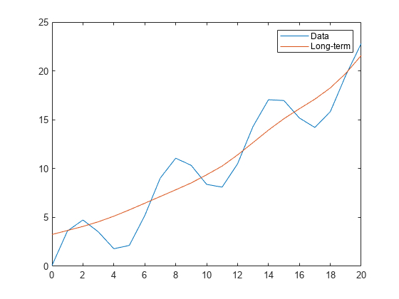
    Compute the long-term trend. Plot the data and the long-term trend.

    LT = trenddecomp(A);
    plot(t,A,t,LT)
    legend("Data","Long-term")

    Figure contains an axes object. The axes object contains 2 objects of type line. These objects represent Data, Long-term.

    Decompose a vector of data into its long-term trend, two seasonal trends, and remainder using singular spectrum analysis.

    Create a vector of data A that contains a long-term trend, two seasonal trends with different periods, and a noise component.

    t = (1:200)';
    trend = 0.001*(t-100).^2;
    period1 = 20;
    period2 = 30;
    seasonal1 = 2*sin(2*pi*t/period1);
    seasonal2 = 0.75*sin(2*pi*t/period2);
    noise = 2*(rand(200,1) - 0.5);
    A = trend + seasonal1 + seasonal2 + noise;

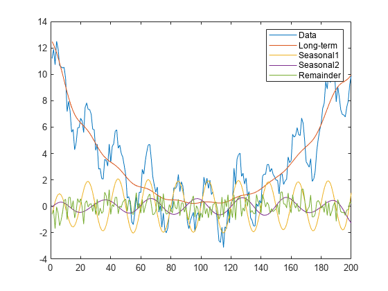
    Decompose the data using the SSA algorithm. Plot the data, the trends, and the remainder.

    [LT,ST,R] = trenddecomp(A);
    plot([A LT ST R]);
    legend("Data","Long-term","Seasonal1","Seasonal2","Remainder")

    Figure contains an axes object. The axes object contains 5 objects of type line. These objects represent Data, Long-term, Seasonal1, Seasonal2, Remainder.

    Decompose tabular data into its long-term trend, two seasonal trends, and remainder using the STL algorithm.

    Create a table T whose variable data contains a long-term trend, two seasonal trends with different periods, and a noise component.

    t = (1:200)';
    trend = 0.001*(t-100).^2;
    period1 = 20;
    period2 = 30;
    seasonal1 = 2*sin(2*pi*t/period1);
    seasonal2 = 0.75*sin(2*pi*t/period2);
    noise = 2*(rand(200,1) - 0.5);
    data = trend + seasonal1 + seasonal2 + noise;
    T = table(data)
    T=200×1 table
         data 
        ______
    
        11.204
        11.896
        10.722
        12.502
        11.939
        10.646
         10.57
        10.479
        10.527
        9.6793
        7.1756
        7.9505
        7.1704
        5.6206
        5.8256
        4.2817
          ⋮


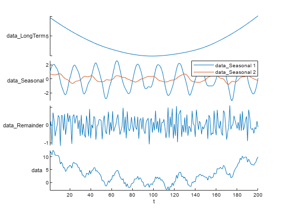
    Decompose the data using the STL algorithm. Plot the data, trends, and remainder.

    D = trenddecomp(T,"stl",[20 30]);
    D = addvars(D,data);
    stackedplot(D)
    xlabel("t")

    Figure contains an object of type stackedplot.

    Input Arguments

    collapse all

    Input array, specified as a numeric vector.

    Data Types: single | double

    Lag value for SSA, specified as a numeric scalar in the interval [3,N/2] where N is the length of the input data. Larger values of lag typically provide more separation of the trends. If the period is known, then specify lag as a multiple of the period.

    Number of seasonal trends for SSA, specified as an integer scalar larger than 0.

    Period for STL, specified as a numeric scalar, numeric vector, duration scalar, or duration vector. When the data has one seasonal trend, specify period as a scalar. When the data has multiple seasonal trends, specify period as a vector whose elements are the periods for each seasonal trend. period can have type duration for timetable input data only.

    Tabular input data, specified as a table or timetable. trenddecomp operates on each table variable separately. Timetables must be uniformly spaced.

    Output Arguments

    collapse all

    Long-term trend, returned as a vector with the same length as the input vector.

    Seasonal trend, returned as a vector or matrix. ST is a vector when the data has one seasonal trend and a matrix when the data has multiple seasonal trends, with each column corresponding to one seasonal trend. The number of rows in ST matches the length of the input vector.

    Remainder, returned as a vector with the same length as the input vector.

    Trends, returned as a table or timetable when the input data is a table or timetable. D contains the long-term trend, seasonal trends, and remainder of the decomposition as separate table variables. For multiple seasonal trends, the number of columns in the resulting variable of D matches the number of seasonal trends.

    Tips

    • An additive decomposition model is appropriate for data where the seasonal variation is relatively constant throughout the time series. If the seasonal variation is proportional to the level of the time series, to use an additive decomposition model, use a log transformation on the data before the decomposition.

    References

    [1] Golyandina, Nina, and Anatoly Zhigljavsky. Singular Spectrum Analysis for Time Series. SpringerBriefs in Statistics. Berlin, Heidelberg: Springer Berlin Heidelberg, 2013. https://doi.org/10.1007/978-3-642-34913-3.

    [2] Cleveland, R.B., W.S. Cleveland, J.E. McRae, and I. Terpenning. “STL: A Seasonal-Trend Decomposition Procedure Based on Loess.” Journal of Official Statistics 6 (1990): 3–73.

    Version History

    Introduced in R2021b
    See Also

    Functions

    Live Editor Tasks