Solve Stiff ODEs
This page contains two examples of solving stiff ordinary differential equations using ode15s. MATLAB® has four solvers designed for stiff ODEs.
ode15sode23sode23tode23tb
For most stiff problems, ode15s performs best. However, ode23s, ode23t, and ode23tb can be more efficient if the problem permits a crude error tolerance.
What is a Stiff ODE?
For some ODE problems, the step size taken by the solver is forced down to an unreasonably small level in comparison to the interval of integration, even in a region where the solution curve is smooth. These step sizes can be so small that traversing a short time interval might require millions of evaluations. This can lead to the solver failing the integration, but even if it succeeds it will take a very long time to do so.
Equations that cause this behavior in ODE solvers are said to be stiff. The problem that stiff ODEs pose is that explicit solvers (such as ode45) are untenably slow in achieving a solution. This is why ode45 is classified as a nonstiff solver along with ode23, ode78, ode89, and ode113.
Solvers that are designed for stiff ODEs, known as stiff solvers, typically do more work per step. The pay-off is that they are able to take much larger steps, and have improved numerical stability compared to the nonstiff solvers.
Solver Options
For stiff problems, specifying the Jacobian matrix using odeset is particularly important. Stiff solvers use the Jacobian matrix  to estimate the local behavior of the ODE as the integration proceeds, so supplying the Jacobian matrix (or, for large sparse systems, its sparsity pattern) is critical for efficiency and reliability. Use the
 Jacobian, JPattern, or Vectorized options of odeset to specify information about the Jacobian. If you do not supply the Jacobian then the solver estimates it numerically using finite differences.
See odeset for a complete listing of other solver options.
Example: Stiff van der Pol Equation
The van der Pol equation is a second order ODE

where  is a scalar parameter. When
  , the resulting system of ODEs is nonstiff and easily solved using
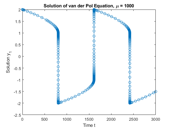
 ode45. However, if you increase  to 1000, then the solution changes dramatically and exhibits oscillation on a much longer time scale. Approximating the solution of the initial value problem becomes more difficult. Because this particular problem is stiff, a solver intended for nonstiff problems, such as
 ode45, is too inefficient to be practical. Use a stiff solver such as ode15s for this problem instead.
Rewrite the van der Pol equation as a system of first-order ODEs by making the substitution  . The resulting system of first-order ODEs is

The vdp1000 function evaluates the van der Pol equation using  .
.
function dydt = vdp1000(t,y)
%VDP1000  Evaluate the van der Pol ODEs for mu = 1000.
%
%   See also ODE15S, ODE23S, ODE23T, ODE23TB.

%   Jacek Kierzenka and Lawrence F. Shampine
%   Copyright 1984-2014 The bat365, Inc.

dydt = [y(2); 1000*(1-y(1)^2)*y(2)-y(1)];
Use the ode15s function to solve the problem with an initial conditions vector of [2; 0], over a time interval of [0 3000]. For scaling reasons, plot only the first component of the solution.
[t,y] = ode15s(@vdp1000,[0 3000],[2; 0]);
plot(t,y(:,1),'-o');
title('Solution of van der Pol Equation, \mu = 1000');
xlabel('Time t');
ylabel('Solution y_1');

The vdpode function also solves the same problem, but it accepts a user-specified value for  . The equations become increasingly stiff as
  increases.
Example: Sparse Brusselator System
The classic Brusselator system of equations is potentially large, stiff, and sparse. The Brusselator system models diffusion in a chemical reaction, and is represented by a system of equations involving  ,
,  ,
,  , and
, and  .
.

The function file brussode solves this set of equations on the time interval [0,10] with  . The initial conditions are

where  for
for  . Therefore, there are
  equations in the system, but the Jacobian
  is a banded matrix with a constant width of 5 if the equations are ordered as
  . As
. As  increases, the problem becomes increasingly stiff, and the Jacobian becomes increasingly sparse.
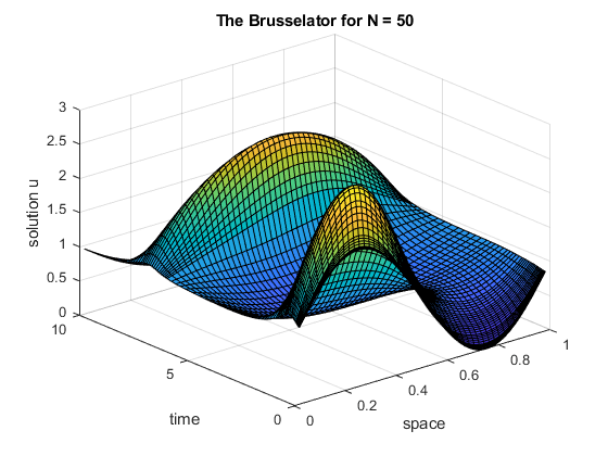
The function call brussode(N), for  , specifies a value for
 N in the system of equations, corresponding to the number of grid points. By default, brussode uses  .
.
brussode contains a few subfunctions:
The nested function
f(t,y)encodes the system of equations for the Brusselator problem, returning a vector.The local function
jpattern(N)returns a sparse matrix of 1s and 0s showing the locations of nonzeros in the Jacobian. This matrix is assigned to theJPatternfield of the options structure. The ODE solver uses this sparsity pattern to generate the Jacobian numerically as a sparse matrix. Supplying this sparsity pattern in the problem significantly reduces the number of function evaluations required to generate the 2N-by-2N Jacobian, from 2N evaluations to just 4.
function brussode(N)
%BRUSSODE  Stiff problem modelling a chemical reaction (the Brusselator).
%   The parameter N >= 2 is used to specify the number of grid points; the
%   resulting system consists of 2N equations. By default, N is 20.  The
%   problem becomes increasingly stiff and increasingly sparse as N is
%   increased.  The Jacobian for this problem is a sparse constant matrix
%   (banded with bandwidth 5).
%
%   The property 'JPattern' is used to provide the solver with a sparse
%   matrix of 1's and 0's showing the locations of nonzeros in the Jacobian
%   df/dy.  By default, the stiff solvers of the ODE Suite generate Jacobians
%   numerically as full matrices.  However, when a sparsity pattern is
%   provided, the solver uses it to generate the Jacobian numerically as a
%   sparse matrix.  Providing a sparsity pattern can significantly reduce the
%   number of function evaluations required to generate the Jacobian and can
%   accelerate integration.  For the BRUSSODE problem, only 4 evaluations of
%   the function are needed to compute the 2N x 2N Jacobian matrix.
%
%   Setting the 'Vectorized' property indicates the function f is
%   vectorized.
%
%   E. Hairer and G. Wanner, Solving Ordinary Differential Equations II,
%   Stiff and Differential-Algebraic Problems, Springer-Verlag, Berlin,
%   1991, pp. 5-8.
%
%   See also ODE15S, ODE23S, ODE23T, ODE23TB, ODESET, FUNCTION_HANDLE.

%   Mark W. Reichelt and Lawrence F. Shampine, 8-30-94
%   Copyright 1984-2014 The bat365, Inc.

% Problem parameter, shared with the nested function.
if nargin<1
   N = 20;
end

tspan = [0; 10];
y0 = [1+sin((2*pi/(N+1))*(1:N)); repmat(3,1,N)];

options = odeset('Vectorized','on','JPattern',jpattern(N));

[t,y] = ode15s(@f,tspan,y0,options);

u = y(:,1:2:end);
x = (1:N)/(N+1);
figure;
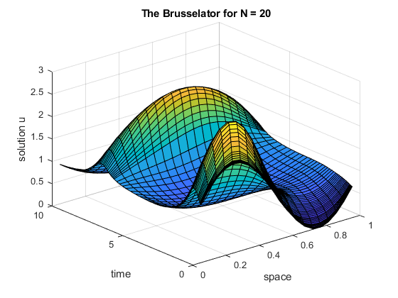
surf(x,t,u);
view(-40,30);
xlabel('space');
ylabel('time');
zlabel('solution u');
title(['The Brusselator for N = ' num2str(N)]);

% -------------------------------------------------------------------------
% Nested function -- N is provided by the outer function.
%

   function dydt = f(t,y)
      % Derivative function
      c = 0.02 * (N+1)^2;
      dydt = zeros(2*N,size(y,2));      % preallocate dy/dt

      % Evaluate the 2 components of the function at one edge of the grid
      % (with edge conditions).
      i = 1;
      dydt(i,:) = 1 + y(i+1,:).*y(i,:).^2 - 4*y(i,:) + c*(1-2*y(i,:)+y(i+2,:));
      dydt(i+1,:) = 3*y(i,:) - y(i+1,:).*y(i,:).^2 + c*(3-2*y(i+1,:)+y(i+3,:));

      % Evaluate the 2 components of the function at all interior grid points.
      i = 3:2:2*N-3;
      dydt(i,:) = 1 + y(i+1,:).*y(i,:).^2 - 4*y(i,:) + ...
         c*(y(i-2,:)-2*y(i,:)+y(i+2,:));
      dydt(i+1,:) = 3*y(i,:) - y(i+1,:).*y(i,:).^2 + ...
         c*(y(i-1,:)-2*y(i+1,:)+y(i+3,:));

      % Evaluate the 2 components of the function at the other edge of the grid
      % (with edge conditions).
      i = 2*N-1;
      dydt(i,:) = 1 + y(i+1,:).*y(i,:).^2 - 4*y(i,:) + c*(y(i-2,:)-2*y(i,:)+1);
      dydt(i+1,:) = 3*y(i,:) - y(i+1,:).*y(i,:).^2 + c*(y(i-1,:)-2*y(i+1,:)+3);
   end
% -------------------------------------------------------------------------

end  % brussode

% ---------------------------------------------------------------------------
% Subfunction -- the sparsity pattern
%

function S = jpattern(N)
% Jacobian sparsity pattern
B = ones(2*N,5);
B(2:2:2*N,2) = zeros(N,1);
B(1:2:2*N-1,4) = zeros(N,1);
S = spdiags(B,-2:2,2*N,2*N);
end
% ---------------------------------------------------------------------------
Solve the Brusselator system for  by running the function
 brussode.
brussode

Solve the system for  by specifying an input to
 brussode.
brussode(50)

See Also
ode15s | ode23s | ode23t | ode23tb
