bat365 Homepage

Lidar 3-D Object Detection Using PointPillars Deep Learning

This example uses:

This example shows how to train a PointPillars network for object detection in point clouds.

Lidar point cloud data can be acquired by a variety of lidar sensors, including Velodyne®, Pandar, and Ouster sensors. These sensors capture 3-D position information about objects in a scene, which is useful for many applications in autonomous driving and augmented reality. However, training robust detectors with point cloud data is challenging because of the sparsity of data per object, object occlusions, and sensor noise. Deep learning techniques have been shown to address many of these challenges by learning robust feature representations directly from point cloud data. One deep learning technique for 3-D object detection is PointPillars [1]. Using a similar architecture to PointNet, the PointPillars network extracts dense, robust features from sparse point clouds called pillars, then uses a 2-D deep learning network with a modified SSD object detection network to estimate joint 3-D bounding boxes, orientations, and class predictions.

Download Lidar Data Set

This example uses a subset of PandaSet [2] that contains 2560 preprocessed organized point clouds. Each point cloud covers $360^{o}$ of view, and is specified as a 64-by-1856 matrix. The point clouds are stored in PCD format and their corresponding ground truth data is stored in the PandaSetLidarGroundTruth.mat file. The file contains 3-D bounding box information for three classes, which are car, truck, and pedestrian. The size of the data set is 5.2 GB.

Download the Pandaset dataset from the given URL using the helperDownloadPandasetData helper function, defined at the end of this example.

doTraining = false;

outputFolder = fullfile(tempdir,'Pandaset');

lidarURL = ['https://ssd.bat365/supportfiles/lidar/data/' ...
    'Pandaset_LidarData.tar.gz'];
helperDownloadPandasetData(outputFolder,lidarURL);

Depending on your Internet connection, the download process can take some time. The code suspends MATLAB® execution until the download process is complete. Alternatively, you can download the data set to your local disk using your web browser and extract the file. If you do so, change the outputFolder variable in the code to the location of the downloaded file. The downloaded file contains Lidar, Cuboids and semanticLabels folders that holds the point clouds, cuboid label and semantic label info respectively

Load Data

Create a file datastore to load the PCD files from the specified path using the pcread function.

path = fullfile(outputFolder,'Lidar');
lidarData = fileDatastore(path,'ReadFcn',@(x) pcread(x));

Load the 3-D bounding box labels of the car and truck objects.

gtPath = fullfile(outputFolder,'Cuboids','PandaSetLidarGroundTruth.mat');
data = load(gtPath,'lidarGtLabels');
Labels = timetable2table(data.lidarGtLabels);
boxLabels = Labels(:,2:3);

Display the full-view point cloud.

figure
ptCld = read(lidarData);
ax = pcshow(ptCld.Location);
set(ax,'XLim',[-50 50],'YLim',[-40 40]);
zoom(ax,2.5);
axis off;

reset(lidarData);

Preprocess Data

The PandaSet data consists of full-view point clouds. For this example, crop the full-view point clouds to front-view point clouds using the standard parameters [1]. These parameters determine the size of the input passed to the network. Select a smaller point cloud range along the x, y, and z-axis to detect objects closer to origin. This also decreases the overall training time of the network.

xMin = 0.0;     % Minimum value along X-axis.
yMin = -39.68;  % Minimum value along Y-axis.
zMin = -5.0;    % Minimum value along Z-axis.
xMax = 69.12;   % Maximum value along X-axis.
yMax = 39.68;   % Maximum value along Y-axis.
zMax = 5.0;     % Maximum value along Z-axis.
xStep = 0.16;   % Resolution along X-axis.
yStep = 0.16;   % Resolution along Y-axis.
dsFactor = 2.0; % Downsampling factor.

% Calculate the dimensions for the pseudo-image.
Xn = round(((xMax - xMin)/xStep));
Yn = round(((yMax - yMin)/yStep));

% Define point cloud parameters.
pointCloudRange = [xMin xMax yMin yMax zMin zMax];
voxelSize = [xStep yStep];

Use the cropFrontViewFromLidarData helper function, attached to this example as a supporting file, to:

Crop the front view from the input full-view point cloud.
Select the box labels that are inside the ROI specified by gridParams.

[croppedPointCloudObj,processedLabels] = cropFrontViewFromLidarData(...
    lidarData,boxLabels,pointCloudRange);

Processing data 100% complete

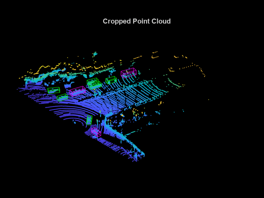
Display the cropped point cloud and the ground truth box labels using the helperDisplay3DBoxesOverlaidPointCloud helper function defined at the end of the example.

pc = croppedPointCloudObj{1,1};
gtLabelsCar = processedLabels.Car{1};
gtLabelsTruck = processedLabels.Truck{1};

helperDisplay3DBoxesOverlaidPointCloud(pc.Location,gtLabelsCar,...
   'green',gtLabelsTruck,'magenta','Cropped Point Cloud');

reset(lidarData);

Create Datastore Objects for Training

Split the data set into training and test sets. Select 70% of the data for training the network and the rest for evaluation.

rng(1);
shuffledIndices = randperm(size(processedLabels,1));
idx = floor(0.7 * length(shuffledIndices));

trainData = croppedPointCloudObj(shuffledIndices(1:idx),:);
testData = croppedPointCloudObj(shuffledIndices(idx+1:end),:);

trainLabels = processedLabels(shuffledIndices(1:idx),:);
testLabels = processedLabels(shuffledIndices(idx+1:end),:);

So that you can easily access the datastores, save the training data as PCD files by using the saveptCldToPCD helper function, attached to this example as a supporting file. You can set writeFiles to "false" if your training data is saved in a folder and is supported by the pcread function.

writeFiles = true;
dataLocation = fullfile(outputFolder,'InputData');
[trainData,trainLabels] = saveptCldToPCD(trainData,trainLabels,...
    dataLocation,writeFiles);

Processing data 100% complete

Create a file datastore using fileDatastore to load PCD files using the pcread function.

lds = fileDatastore(dataLocation,'ReadFcn',@(x) pcread(x));

Createa box label datastore using boxLabelDatastore for loading the 3-D bounding box labels.

bds = boxLabelDatastore(trainLabels);

Use the combine function to combine the point clouds and 3-D bounding box labels into a single datastore for training.

cds = combine(lds,bds);

Data Augmentation

This example uses ground truth data augmentation and several other global data augmentation techniques to add more variety to the training data and corresponding boxes. For more information on typical data augmentation techniques used in 3-D object detection workflows with lidar data, see the Data Augmentations for Lidar Object Detection Using Deep Learning.

Read and display a point cloud before augmentation using the helperDisplay3DBoxesOverlaidPointCloud helper function, defined at the end of the example..

augData = read(cds);
augptCld = augData{1,1};
augLabels = augData{1,2};
augClass = augData{1,3};

labelsCar = augLabels(augClass=='Car',:);
labelsTruck = augLabels(augClass=='Truck',:);

helperDisplay3DBoxesOverlaidPointCloud(augptCld.Location,labelsCar,'green',...
    labelsTruck,'magenta','Before Data Augmentation');

reset(cds);

Use the sampleLidarData function to sample 3-D bounding boxes and their corresponding points from the training data.

classNames = {'Car','Truck'};
sampleLocation = fullfile(outputFolder,'GTsamples');
[ldsSampled,bdsSampled] = sampleLidarData(cds,classNames,'MinPoints',20,...                  
                            'Verbose',false,'WriteLocation',sampleLocation);
cdsSampled = combine(ldsSampled,bdsSampled);

Use the pcBboxOversample function to randomly add a fixed number of car and truck class objects to every point cloud. Use the transform function to apply the ground truth and custom data augmentations to the training data.

numObjects = [10 10];
cdsAugmented = transform(cds,@(x)pcBboxOversample(x,cdsSampled,classNames,numObjects));

Apply these additional data augmentation techniques to every point cloud.

Random flipping along the x-axis
Random scaling by 5 percent
Random rotation along the z-axis from [-pi/4, pi/4]
Random translation by [0.2, 0.2, 0.1] meters along the x-, y-, and z-axis respectively

cdsAugmented = transform(cdsAugmented,@(x)augmentData(x));

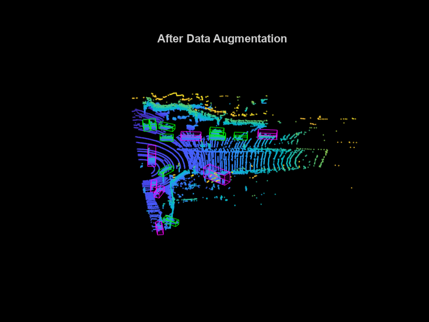
Display an augmented point cloud along with the ground truth augmented boxes using the helperDisplay3DBoxesOverlaidPointCloud helper function, defined at the end of the example.

augData = read(cdsAugmented);
augptCld = augData{1,1};
augLabels = augData{1,2};
augClass = augData{1,3};

labelsCar = augLabels(augClass=='Car',:);
labelsTruck = augLabels(augClass=='Truck',:);

helperDisplay3DBoxesOverlaidPointCloud(augptCld.Location,labelsCar,'green',...
    labelsTruck,'magenta','After Data Augmentation');

reset(cdsAugmented);

Create PointPillars Object Detector

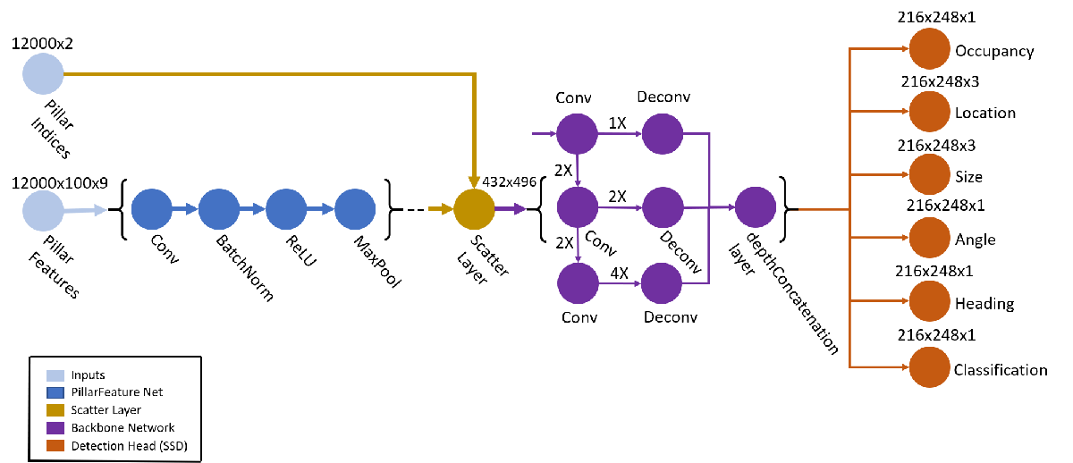
Use the pointPillarsObjectDetector function to create a PointPillars object detection network. For more information on PointPillars network, see Get Started with PointPillars.

The diagram shows the network architecture of a PointPillars object detector. You can use the Deep Network Designer (Deep Learning Toolbox) App to create a PointPillars network.

The pointPillarsObjectDetector function requires you to specify several inputs that parameterize the PointPillars network:

Class names
Anchor boxes
Point cloud range
Voxel size
Number of prominent pillars
Number of points per pillar

% Define the number of prominent pillars.
P = 12000; 

% Define the number of points per pillar.
N = 100;

Estimate the anchor boxes from training data using calculateAnchorsPointPillars helper function, attached to this example as a supporting file.

anchorBoxes = calculateAnchorsPointPillars(trainLabels);
classNames = trainLabels.Properties.VariableNames;

Define the PointPillars detector.

detector = pointPillarsObjectDetector(pointCloudRange,classNames,anchorBoxes,...
    'VoxelSize',voxelSize,'NumPillars',P,'NumPointsPerPillar',N);

Train Pointpillars Object Detector

Specify the network training parameters using the trainingOptions (Deep Learning Toolbox) function. Set 'CheckpointPath' to a temporary location to enable saving of partially trained detectors during the training process. If training is interrupted, you can resume training from the saved checkpoint.

Train the detector using a CPU or GPU. Using a GPU requires Parallel Computing Toolbox™ and a CUDA® enabled NVIDIA® GPU. For more information, see GPU Computing Requirements (Parallel Computing Toolbox). To automatically detect if you have a GPU available, set executionEnvironment to "auto". If you do not have a GPU, or do not want to use one for training, set executionEnvironment to "cpu". To ensure the use of a GPU for training, set executionEnvironment to "gpu".

executionEnvironment = "auto";
if canUseParallelPool
    dispatchInBackground = true;
else
    dispatchInBackground = false;
end

options = trainingOptions('adam',...
    'Plots',"none",...
    'MaxEpochs',60,...
    'MiniBatchSize',3,...
    'GradientDecayFactor',0.9,...
    'SquaredGradientDecayFactor',0.999,...
    'LearnRateSchedule',"piecewise",...
    'InitialLearnRate',0.0002,...
    'LearnRateDropPeriod',15,...
    'LearnRateDropFactor',0.8,...
    'ExecutionEnvironment',executionEnvironment,...
    'DispatchInBackground',dispatchInBackground,...
    'BatchNormalizationStatistics','moving',...
    'ResetInputNormalization',false,...
    'CheckpointPath',tempdir);

Use the trainPointPillarsObjectDetector function to train the PointPillars object detector if doTraining is "true". Otherwise, load a pretrained detector.

Note: The pretrained network pretrainedPointPillarsDetector.mat is trained on point cloud data captured by a Pandar 64 sensor where the ego vehicle direction is along positive y-axis.

To generate accurate detections using this pretrained network on a custom dataset,

Transform your point cloud data such that the ego vehicle moves along positive y-axis.
Restructure your data with Padar 64 parameters by using the pcorganize function.

if doTraining    
    [detector,info] = trainPointPillarsObjectDetector(cdsAugmented,detector,options);
else
    pretrainedDetector = load('pretrainedPointPillarsDetector.mat','detector');
    detector = pretrainedDetector.detector;
end

Generate Detections

Use the trained network to detect objects in the test data:

Read the point cloud from the test data.
Run the detector on the test point cloud to get the predicted bounding boxes and confidence scores.
Display the point cloud with bounding boxes using the helperDisplay3DBoxesOverlaidPointCloud helper function, defined at the end of the example.

ptCloud = testData{45,1};
gtLabels = testLabels(45,:);

% Specify the confidence threshold to use only detections with
% confidence scores above this value.
confidenceThreshold = 0.5;
[box,score,labels] = detect(detector,ptCloud,'Threshold',confidenceThreshold);

boxlabelsCar = box(labels'=='Car',:);
boxlabelsTruck = box(labels'=='Truck',:);

% Display the predictions on the point cloud.
helperDisplay3DBoxesOverlaidPointCloud(ptCloud.Location,boxlabelsCar,'green',...
    boxlabelsTruck,'magenta','Predicted Bounding Boxes');

Evaluate Detector Using Test Set

Evaluate the trained object detector on a large set of point cloud data to measure the performance.

numInputs = 50;

% Generate rotated rectangles from the cuboid labels.
bds = boxLabelDatastore(testLabels(1:numInputs,:));
groundTruthData = transform(bds,@(x)createRotRect(x));

% Set the threshold values.
nmsPositiveIoUThreshold = 0.5;
confidenceThreshold = 0.25;

detectionResults = detect(detector,testData(1:numInputs,:),...
    'Threshold',confidenceThreshold);

% Convert the bounding boxes to rotated rectangles format and calculate
% the evaluation metrics.
for i = 1:height(detectionResults)
    box = detectionResults.Boxes{i};
    detectionResults.Boxes{i} = box(:,[1,2,4,5,9]);
end

metrics = evaluateDetectionAOS(detectionResults,groundTruthData,...
    nmsPositiveIoUThreshold);
disp(metrics(:,1:2))

               AOS        AP   
             _______    _______

    Car      0.74377    0.75569
    Truck    0.60989    0.61157

Helper Functions

function helperDownloadPandasetData(outputFolder,lidarURL)
% Download the data set from the given URL to the output folder.

    lidarDataTarFile = fullfile(outputFolder,'Pandaset_LidarData.tar.gz');
    
    if ~exist(lidarDataTarFile,'file')
        mkdir(outputFolder);
        
        disp('Downloading PandaSet Lidar driving data (5.2 GB)...');
        websave(lidarDataTarFile,lidarURL);
        untar(lidarDataTarFile,outputFolder);
    end
    
    % Extract the file.
    if (~exist(fullfile(outputFolder,'Lidar'),'dir'))...
            &&(~exist(fullfile(outputFolder,'Cuboids'),'dir'))
        untar(lidarDataTarFile,outputFolder);
    end

end

function helperDisplay3DBoxesOverlaidPointCloud(ptCld,labelsCar,carColor,...
    labelsTruck,truckColor,titleForFigure)
% Display the point cloud with different colored bounding boxes for different
% classes.
    figure;
    ax = pcshow(ptCld);
    showShape('cuboid',labelsCar,'Parent',ax,'Opacity',0.1,...
        'Color',carColor,'LineWidth',0.5);
    hold on;
    showShape('cuboid',labelsTruck,'Parent',ax,'Opacity',0.1,...
        'Color',truckColor,'LineWidth',0.5);
    title(titleForFigure);
    zoom(ax,1.5);
end

References

[1] Lang, Alex H., Sourabh Vora, Holger Caesar, Lubing Zhou, Jiong Yang, and Oscar Beijbom. "PointPillars: Fast Encoders for Object Detection From Point Clouds." In 2019 IEEE/CVF Conference on Computer Vision and Pattern Recognition (CVPR), 12689-12697. Long Beach, CA, USA: IEEE, 2019. https://doi.org/10.1109/CVPR.2019.01298.

[2] Hesai and Scale. PandaSet. https://scale.com/open-datasets/pandaset.