paretosearch
Find points in Pareto set
Syntax
Description
x = paretosearch(fun,nvars,A,b,Aeq,beq,lb,ub)x, so that x is always in the range
lb ≤ x ≤ ub.
If no linear equalities exist, set Aeq = [] and beq =
[]. If x(i) has no lower bound, set lb(i)
= -Inf. If x(i) has no upper bound, set
ub(i) = Inf.
x = paretosearch(fun,nvars,A,b,Aeq,beq,lb,ub,nonlcon)c(x) defined in
nonlcon. The paretosearch function finds
nondominated points such that c(x) ≤ 0. If no bounds
exist, set lb = [], ub = [], or both.
Note
Currently, paretosearch does not support nonlinear equality
constraints ceq(x) = 0.
Examples
Find Pareto Front
Find points on the Pareto front of a two-objective function of a two-dimensional variable.
fun = @(x)[norm(x-[1,2])^2;norm(x+[2,1])^2];
rng default % For reproducibility
x = paretosearch(fun,2);
Pareto set found that satisfies the constraints.

Optimization completed because the relative change in the volume of the Pareto set
is less than 'options.ParetoSetChangeTolerance' and constraints are satisfied to within
'options.ConstraintTolerance'.
Plot the solution as a scatter plot.
plot(x(:,1),x(:,2),'m*')
xlabel('x(1)')
ylabel('x(2)')
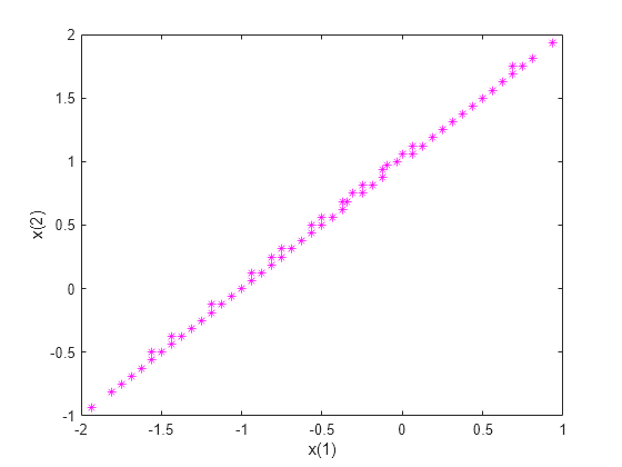
Theoretically, the solution of this problem is a straight line from [-2,-1] to [1,2]. paretosearch returns evenly-spaced points close to this line.
Create Pareto Front with Linear Constraints
Create a Pareto front for a two-objective problem in two dimensions subject to the linear constraint x(1) + x(2) <= 1.
fun = @(x)[norm(x-[1,2])^2;norm(x+[2,1])^2];
A = [1,1];
b = 1;
rng default % For reproducibility
x = paretosearch(fun,2,A,b);
Pareto set found that satisfies the constraints.

Optimization completed because the relative change in the volume of the Pareto set
is less than 'options.ParetoSetChangeTolerance' and constraints are satisfied to within
'options.ConstraintTolerance'.
Plot the solution as a scatter plot.
plot(x(:,1),x(:,2),'m*')
xlabel('x(1)')
ylabel('x(2)')
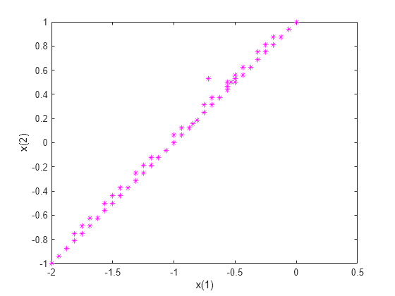
Theoretically, the solution of this problem is a straight line from [-2,-1] to [0,1]. paretosearch returns evenly-spaced points close to this line.
Create Pareto Front with Bounds
Create a Pareto front for a two-objective problem in two dimensions subject to the bounds x(1) >= 0 and x(2) <= 1.
fun = @(x)[norm(x-[1,2])^2;norm(x+[2,1])^2];
lb = [0,-Inf]; % x(1) >= 0
ub = [Inf,1]; % x(2) <= 1
rng default % For reproducibility
x = paretosearch(fun,2,[],[],[],[],lb,ub);
Pareto set found that satisfies the constraints.

Optimization completed because the relative change in the volume of the Pareto set
is less than 'options.ParetoSetChangeTolerance' and constraints are satisfied to within
'options.ConstraintTolerance'.
Plot the solution as a scatter plot.
plot(x(:,1),x(:,2),'m*')
xlabel('x(1)')
ylabel('x(2)')
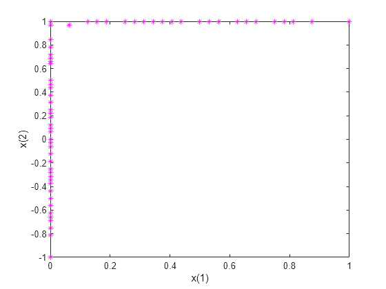
All of the solution points are on the constraint boundaries x(1) = 0 or x(2) = 1.
Create Pareto Front with Nonlinear Constraints
Create a Pareto front for a two-objective problem in two dimensions subject to bounds -1.1 <= x(i) <= 1.1 and the nonlinear constraint norm(x)^2 <= 1.2. The nonlinear constraint function appears at the end of this example, and works if you run this example as a live script. To run this example otherwise, include the nonlinear constraint function as a file on your MATLAB® path.
To better see the effect of the nonlinear constraint, set options to use a large Pareto set size.
rng default % For reproducibility
fun = @(x)[norm(x-[1,2])^2;norm(x+[2,1])^2];
lb = [-1.1,-1.1];
ub = [1.1,1.1];
options = optimoptions('paretosearch','ParetoSetSize',200);
x = paretosearch(fun,2,[],[],[],[],lb,ub,@circlecons,options);
Pareto set found that satisfies the constraints.

Optimization completed because the relative change in the volume of the Pareto set
is less than 'options.ParetoSetChangeTolerance' and constraints are satisfied to within
'options.ConstraintTolerance'.
Plot the solution as a scatter plot. Include a plot of the circular constraint boundary.
figure
plot(x(:,1),x(:,2),'k*')
xlabel('x(1)')
ylabel('x(2)')
hold on
rectangle('Position',[-1.2 -1.2 2.4 2.4],'Curvature',1,'EdgeColor','r')
xlim([-1.2,0.5])
ylim([-0.5,1.2])
axis square
hold off
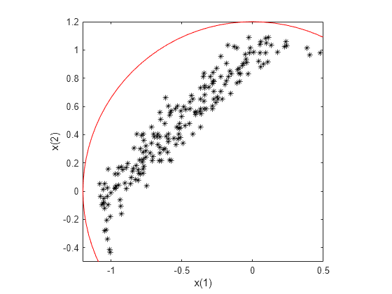
The solution points that have positive x(1) values or negative x(2) values are close to the nonlinear constraint boundary.
function [c,ceq] = circlecons(x)
ceq = [];
c = norm(x)^2 - 1.2;
end
Find Pareto Front Using Options
To monitor the progress of paretosearch, specify the 'psplotparetof' plot function.
fun = @(x)[norm(x-[1,2])^2;norm(x+[2,1])^2];
options = optimoptions('paretosearch','PlotFcn','psplotparetof');
lb = [-4,-4];
ub = -lb;
x = paretosearch(fun,2,[],[],[],[],lb,ub,[],options);
Pareto set found that satisfies the constraints.

Optimization completed because the relative change in the volume of the Pareto set
is less than 'options.ParetoSetChangeTolerance' and constraints are satisfied to within
'options.ConstraintTolerance'.
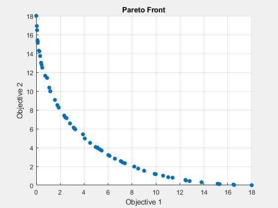
The solution looks like a quarter-circular arc with radius 18, which can be shown to be the analytical solution.
Find Pareto Front in Function Space and Parameter Space
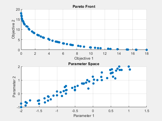
Obtain the Pareto front in both function space and parameter space by calling paretosearch with both the x and fval outputs. Set options to plot the Pareto set in both function space and parameter space.
fun = @(x)[norm(x-[1,2])^2;norm(x+[2,1])^2];
lb = [-4,-4];
ub = -lb;
options = optimoptions('paretosearch','PlotFcn',{'psplotparetof' 'psplotparetox'});
rng default % For reproducibility
[x,fval] = paretosearch(fun,2,[],[],[],[],lb,ub,[],options);
Pareto set found that satisfies the constraints.

Optimization completed because the relative change in the volume of the Pareto set
is less than 'options.ParetoSetChangeTolerance' and constraints are satisfied to within
'options.ConstraintTolerance'.

The analytical solution in objective function space is a quarter-circular arc of radius 18. In parameter space, the analytical solution is a straight line from [-2,-1] to [1,2]. The solution points are close to the analytical curves.
Monitor Pareto Set Solution
Set options to monitor the Pareto set solution process. Also, obtain more outputs from paretosearch to enable you to understand the solution process.
options = optimoptions('paretosearch','Display','iter',...
    'PlotFcn',{'psplotparetof' 'psplotparetox'});
fun = @(x)[norm(x-[1,2])^2;norm(x+[2,1])^2];
lb = [-4,-4];
ub = -lb;
rng default % For reproducibility
[x,fval,exitflag,output] = paretosearch(fun,2,[],[],[],[],lb,ub,[],options);
Iter   F-count   NumSolutions  Spread       Volume
   0        60        11          -         3.7872e+02
   1       386        12       7.6126e-01   3.4654e+02
   2       702        27       9.5232e-01   2.9452e+02
   3      1029        27       6.6332e-02   2.9904e+02
   4      1357        36       1.3874e-01   3.0070e+02
   5      1690        37       1.5379e-01   3.0200e+02
   6      2014        50       1.7828e-01   3.0252e+02
   7      2214        59       1.8536e-01   3.0320e+02
   8      2344        60       1.9435e-01   3.0361e+02
   9      2464        60       2.1055e-01   3.0388e+02

Pareto set found that satisfies the constraints.

Optimization completed because the relative change in the volume of the Pareto set
is less than 'options.ParetoSetChangeTolerance' and constraints are satisfied to within
'options.ConstraintTolerance'.
Examine the additional outputs.
fprintf('Exit flag %d.\n',exitflag)Exit flag 1.
disp(output)
         iterations: 10
          funccount: 2464
             volume: 303.6076
    averagedistance: 0.0250
             spread: 0.2105
      maxconstraint: 0
            message: 'Pareto set found that satisfies the constraints. ...'
           rngstate: [1x1 struct]
Obtain Pareto Front Residuals
Obtain and examine the Pareto front constraint residuals. Create a problem with the linear inequality constraint sum(x) <= -1/2 and the nonlinear inequality constraint norm(x)^2 <= 1.2. For improved accuracy, use 200 points on the Pareto front, and a ParetoSetChangeTolerance of 1e-7, and give the natural bounds -1.2 <= x(i) <= 1.2.
The nonlinear constraint function appears at the end of this example, and works if you run this example as a live script. To run this example otherwise, include the nonlinear constraint function as a file on your MATLAB® path.
fun = @(x)[norm(x-[1,2])^2;norm(x+[2,1])^2];
A = [1,1];
b = -1/2;
lb = [-1.2,-1.2];
ub = -lb;
nonlcon = @circlecons;
rng default % For reproducibility
options = optimoptions('paretosearch','ParetoSetChangeTolerance',1e-7,...
    'PlotFcn',{'psplotparetof' 'psplotparetox'},'ParetoSetSize',200);
Call paretosearch using all outputs.
[x,fval,exitflag,output,residuals] = paretosearch(fun,2,A,b,[],[],lb,ub,nonlcon,options);
Pareto set found that satisfies the constraints.

Optimization completed because the relative change in the volume of the Pareto set
is less than 'options.ParetoSetChangeTolerance' and constraints are satisfied to within
'options.ConstraintTolerance'.
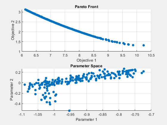
The inequality constraints reduce the size of the Pareto set compared to an unconstrained set. Examine the returned residuals.
fprintf('The maximum linear inequality constraint residual is %f.\n',max(residuals.ineqlin))The maximum linear inequality constraint residual is 0.000000.
fprintf('The maximum nonlinear inequality constraint residual is %f.\n',max(residuals.ineqnonlin))The maximum nonlinear inequality constraint residual is -0.000537.
The maximum returned residuals are negative, meaning that all the returned points are feasible. The maximum returned residuals are close to zero, meaning that each constraint is active for some points.
function [c,ceq] = circlecons(x)
ceq = [];
c = norm(x)^2 - 1.2;
end
Input Arguments
fun — Objective functions to optimize
function handle | function name
Objective functions to optimize, specified as a function handle or function name.
fun is a function that accepts a real row vector of
doubles x of length nvars and
returns a real vector F(x) of objective function values.
For details on writing fun, see Compute Objective Functions.
If you set the UseVectorized option to
true, then fun accepts a matrix of
size n-by-nvars, where the matrix
represents n individuals. fun returns
a matrix of size n-by-m, where
m is the number of objective functions. See Vectorize the Fitness Function.
Example: @(x)[sin(x),cos(x)]
Data Types: char | function_handle | string
nvars — Number of variables
positive integer
Number of variables, specified as a positive integer. The solver passes row vectors of length
nvars to fun.
Example: 4
Data Types: double
A — Linear inequality constraints
real matrix
Linear inequality constraints, specified as a real matrix. A is an M-by-nvars matrix, where M is the number of inequalities.
A encodes the M linear inequalities
A*x <= b,
where x is the column vector of nvars variables x(:), and b is a column vector with M elements.
For example, to specify
x1 + 2x2 ≤ 10
3x1 + 4x2 ≤ 20
5x1 + 6x2 ≤ 30,
give these constraints:
A = [1,2;3,4;5,6];
b = [10;20;30];
Example: To specify that the control variables sum to 1 or less, give the constraints
A = ones(1,N) and b = 1.
Data Types: double
b — Linear inequality constraints
real vector
Linear inequality constraints, specified as a real vector. b is an M-element vector related to the A matrix. If you pass b as a row vector, solvers internally convert b to the column vector b(:).
b encodes the M linear inequalities
A*x <= b,
where x is the column vector of N variables x(:), and A is a matrix of size M-by-N.
For example, to specify
x1 + 2x2 ≤ 10
3x1 + 4x2 ≤ 20
5x1 + 6x2 ≤ 30,
give these constraints:
A = [1,2;3,4;5,6];
b = [10;20;30];
Example: To specify that the control variables sum to 1 or less, give the constraints
A = ones(1,N) and b = 1.
Data Types: double
Aeq — Linear equality constraints
real matrix
Linear equality constraints, specified as a real matrix. Aeq is an Me-by-nvars matrix, where Me is the number of equalities.
Aeq encodes the Me linear equalities
Aeq*x = beq,
where x is the column vector of N variables x(:), and beq is a column vector with Me elements.
For example, to specify
x1
+ 2x2 +
3x3 =
10
2x1
+ 4x2 +
x3 =
20,
give these constraints:
Aeq = [1,2,3;2,4,1];
beq = [10;20];
Example: To specify that the control variables sum to 1, give the constraints Aeq =
ones(1,N) and beq = 1.
Data Types: double
beq — Linear equality constraints
real vector
Linear equality constraints, specified as a real vector. beq is an Me-element vector related to the Aeq matrix. If you pass beq as a row vector, solvers internally convert beq to the column vector beq(:).
beq encodes the Me linear equalities
Aeq*x = beq,
where x is the column vector of N variables x(:), and Aeq is a matrix of size Meq-by-N.
For example, to specify
x1
+ 2x2 +
3x3 =
10
2x1
+ 4x2 +
x3 =
20,
give these constraints:
Aeq = [1,2,3;2,4,1];
beq = [10;20];
Example: To specify that the control variables sum to 1, give the constraints Aeq =
ones(1,N) and beq = 1.
Data Types: double
lb — Lower bounds
[] (default) | real vector or array
Lower bounds, specified as a real vector or array of doubles. lb represents
the lower bounds element-wise in
lb ≤ x ≤ ub.
Internally, paretosearch converts an array lb to the
vector lb(:).
Example: lb = [0;-Inf;4] means x(1) ≥ 0, x(3) ≥ 4.
Data Types: double
ub — Upper bounds
[] (default) | real vector or array
Upper bounds, specified as a real vector or array of doubles. ub represents
the upper bounds element-wise in
lb ≤ x ≤ ub.
Internally, paretosearch converts an array ub to the
vector ub(:).
Example: ub = [Inf;4;10] means x(2) ≤ 4, x(3) ≤ 10.
Data Types: double
nonlcon — Nonlinear constraints
function handle | function name
Nonlinear constraints, specified as a function handle or function name.
nonlcon is a function that accepts a row vector
x and returns two row vectors,
c(x) and ceq(x).
c(x)is the row vector of nonlinear inequality constraints atx. Theparetosearchfunction attempts to satisfyc(x) <= 0for all entries ofc.ceq(x)must return[], because currentlyparetosearchdoes not support nonlinear equality constraints.
If you set the UseVectorized option to
true, then nonlcon accepts a
matrix of size n-by-nvars, where the
matrix represents n individuals.
nonlcon returns a matrix of size
n-by-mc in the first argument,
where mc is the number of nonlinear inequality
constraints. See Vectorize the Fitness Function.
For example,
x = paretosearch(@myfun,nvars,A,b,Aeq,beq,lb,ub,@mycon),
where mycon is a MATLAB® function such as the following:
function [c,ceq] = mycon(x)
c = ...     % Compute nonlinear inequalities at x.
ceq = []    % No nonlinear equalities at x.
For more information, see Nonlinear Constraints.
Data Types: char | function_handle | string
options — Optimization options
output of optimoptions | structure
Optimization options, specified as the output of optimoptions or as a
structure.
{} denotes the default value. See option details in
Pattern Search Options.
Options for paretosearch
| Option | Description | Values |
|---|---|---|
| Tolerance on constraints. For an options structure, use | Nonnegative scalar | |
| Level of display. | 'off' | 'iter' | 'diagnose' | {'final'} |
| Initial points for
| Matrix with |
| Maximum number of objective function evaluations. For an options structure, use | Nonnegative integer | |
| Maximum number of iterations. For an options structure, use | Nonnegative integer | |
| Total time (in seconds) allowed for optimization. For an options structure, use | Nonnegative scalar | |
| Tolerance on the mesh size. For an options structure, use
| Nonnegative scalar | |
| Minimum fraction of the pattern to poll. | Scalar from 0 through 1 | |
| Function that an optimization function calls at each iteration. Specify as a function handle or a cell array of function handles. For an options structure, use | |
| The solver stops when the relative change in a stopping measure
over a window of iterations is less than or equal to
See Definitions for paretosearch Algorithm. The solver stops when the relative change in any
applicable measure is less than
Note Setting | Nonnegative scalar | |
| Number of points in the Pareto set. | Positive integer | |
| Plots of output from the pattern search. Specify as the name of a built-in plot function, a function handle, or a cell array of names of built-in plot functions or function handles. For an options structure, use
|
With multiple objectives:
With a single
objective: |
| Polling strategy used in the pattern search. Note You cannot use MADS polling when the problem has linear equality constraints. |
|
| Compute objective and nonlinear constraint functions in parallel. See Vectorized and Parallel Options and How to Use Parallel Processing in Global Optimization Toolbox. Note You must set Beginning in R2019a, when you set the
|
|
| Specifies whether functions are vectorized. See Vectorized and Parallel Options and Vectorize the Objective and Constraint Functions. Note You must set For an options structure, use |
|
Example: options =
optimoptions('paretosearch','Display','none','UseParallel',true)
problem — Problem structure
structure
Problem structure, specified as a structure with the following fields:
objective— Objective functionnvars— Number of variablesAineq— Matrix for linear inequality constraintsbineq— Vector for linear inequality constraintsAeq— Matrix for linear equality constraintsbeq— Vector for linear equality constraintslb— Lower bound forxub— Upper bound forxnonlcon— Nonlinear constraint functionsolver—'paretosearch'options— Options created withoptimoptionsrngstate— Optional field to reset the state of the random number generator
Note
All fields in problem are required, except for
rngstate, which is optional.
Data Types: struct
Output Arguments
x — Pareto points
m-by-nvars array
Pareto points, returned as an m-by-nvars array, where
m is the number of points on the Pareto front. Each row of
x represents one point on the Pareto front.
fval — Function values on Pareto front
m-by-nf array
Function values on the Pareto front, returned as an
m-by-nf array.
m is the number of points on the Pareto front, and
nf is the number of objective functions. Each row of
fval represents the function values at one Pareto
point in x.
exitflag — Reason paretosearch stopped
integer
Reason paretosearch stopped, returned as one of the
integer values in this table.
| Exit Flag | Stopping Condition |
|---|---|
1 | One of the following conditions is met.
|
0 | Number of iterations exceeds
options.MaxIterations, or the number
of function evaluations exceeds
options.MaxFunctionEvaluations. |
-1 | Optimization is stopped by an output function or plot function. |
-2 | Solver cannot find a point satisfying all the constraints. |
-5 | Optimization time exceeds
options.MaxTime. |
output — Information about the optimization process
structure
Information about the optimization process, returned as a structure with these fields:
iterations— Total number of iterations.funccount— Total number of function evaluations.volume— Hyper-volume of the set formed from the Pareto points in function space. See Definitions for paretosearch Algorithm.averagedistance— Average distance measure of the Pareto points in function space. See Definitions for paretosearch Algorithm.spread— Average spread measure of the Pareto points. See Definitions for paretosearch Algorithm.maxconstraint— Maximum constraint violation, if any.message— Reason why the algorithm terminated.rngstate— State of the MATLAB random number generator just before the algorithm starts. You can use the values inrngstateto reproduce the output when you use a random poll method such as'MADSPositiveBasis2N'or when you use the default quasirandom method of creating the initial population. See Reproduce Results, which discusses the identical technique forga.
residuals — Constraint residuals at x
structure
Constraint residuals at x, returned as a structure
with these fields (a glossary of the field size terms and entries follows
the table).
| Field Name | Field Size | Entries |
|---|---|---|
lower | m-by-nvars | lb – x |
upper | m-by-nvars | x – ub |
ineqlin | m-by-ncon | A*x - b |
eqlin | m-by-ncon | |Aeq*x - b| |
ineqnonlin | m-by-ncon | c(x) |
m— Number of returned pointsxon the Pareto frontnvars— Number of control variablesncon— Number of constraints of the relevant type (such as number of rows ofAor number of returned nonlinear equalities)c(x)— Numeric values of the nonlinear constraint functions
More About
Nondominated
Nondominated points, also called noninferior points, are points for which no other point has lower values of all objective functions. In other words, for nondominated points, none of the objective function values can be improved (lowered) without raising other objective function values. See What Is Multiobjective Optimization?.
Algorithms
paretosearch uses a pattern search to search for points on the
Pareto front. For details, see paretosearch Algorithm.
Alternative Functionality
App
The Optimize Live Editor task provides a visual interface for paretosearch.
Extended Capabilities
Automatic Parallel Support
Accelerate code by automatically running computation in parallel using Parallel Computing Toolbox™.
To run in parallel, set the 'UseParallel' option to true.
options = optimoptions('solvername','UseParallel',true)
For more information, see How to Use Parallel Processing in Global Optimization Toolbox.
Version History
Introduced in R2018b
MATLAB Command
You clicked a link that corresponds to this MATLAB command:
Run the command by entering it in the MATLAB Command Window. Web browsers do not support MATLAB commands.

Select a Web Site
Choose a web site to get translated content where available and see local events and offers. Based on your location, we recommend that you select: .
You can also select a web site from the following list
How to Get Best Site Performance
Select the China site (in Chinese or English) for best site performance. Other bat365 country sites are not optimized for visits from your location.
Americas
- América Latina (Español)
- Canada (English)
- United States (English)
Europe
- Belgium (English)
- Denmark (English)
- Deutschland (Deutsch)
- España (Español)
- Finland (English)
- France (Français)
- Ireland (English)
- Italia (Italiano)
- Luxembourg (English)
- Netherlands (English)
- Norway (English)
- Österreich (Deutsch)
- Portugal (English)
- Sweden (English)
- Switzerland
- United Kingdom (English)
Asia Pacific
- Australia (English)
- India (English)
- New Zealand (English)
- 中国
- 日本Japanese (日本語)
- 한국Korean (한국어)