Time Series Prediction in Simulink Using Deep Learning Network
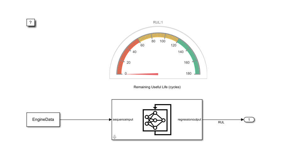
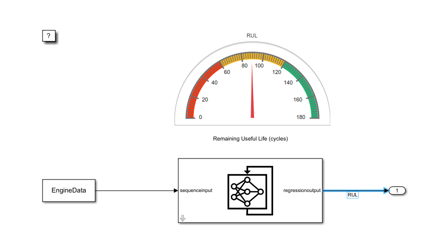
This example shows how to use an LSTM deep learning network inside a Simulink® model to predict the remaining useful life (RUL) of an engine. You include the network inside the Simulink model by using a Stateful Predict block, which predicts the RUL at every simulation step.
This example uses data from the Turbofan Engine Degradation Simulation Data Set as described in [1]. The example uses a trained LSTM network to predict the RUL of an engine (predictive maintenance), measured in cycles, given time series data representing various sensors in the engine. The data used to train the network contains simulated time series data for 100 engines. Each sequence has 17 features of varying length and corresponds to a full run to failure (RTF) instance. For more information on how to train the network, see Sequence-to-Sequence Regression Using Deep Learning.
Download Data
Download and unzip the Turbofan Engine Degradation Simulation data set.
Each time series of the Turbofan Engine Degradation Simulation data set represents a different engine. Each engine starts with unknown degrees of initial wear and manufacturing variation. The engine is operating normally at the start of each time series, and develops a fault at some point during the series. In the training set, the fault grows in magnitude until system failure.
The data contains a ZIP-compressed text files with 26 columns of numbers, separated by spaces. Each row is a snapshot of data taken during a single operational cycle, and each column is a different variable. The columns correspond to the following:
Column 1 – Unit number
Column 2 – Time in cycles
Columns 3–5 – Operational settings
Columns 6–26 – Sensor measurements 1–21
Create a directory to store the Turbofan Engine Degradation Simulation data set.
dataFolder = "data";
if ~exist(dataFolder,"dir")
    mkdir(dataFolder);
end
Download and extract the Turbofan Engine Degradation Simulation data set.
filename = matlab.internal.examples.downloadSupportFile("nnet","data/TurbofanEngineDegradationSimulationData.zip");
unzip(filename,dataFolder)
Prepare Data
Load the data using the processTurboFanDataTrain helper function. The processTurboFanDataTrain function extracts the data from filenamePredictors and returns the cell array XTrain, which contains the training predictor data.
filenamePredictors = fullfile(dataFolder,"train_FD001.txt");
[XTrain] = processTurboFanDataTrain(filenamePredictors);
Remove Features with Constant Values
Since the network was trained with features that do not remain constant for all time steps, features with constant values for all time steps need to be removed for prediction. Find the rows of data that have the same minimum and maximum values, and remove the rows.
m = min([XTrain{:}],[],2);
M = max([XTrain{:}],[],2);
idxConstant = M == m;

for i = 1:numel(XTrain)
    XTrain{i}(idxConstant,:) = [];
end
Normalize Training Predictors
Normalize the training predictors to have zero mean and unit variance. To calculate the mean and standard deviation over all observations, concatenate the sequence data horizontally.
mu = mean([XTrain{:}],2);
sig = std([XTrain{:}],0,2);

for i = 1:numel(XTrain)
    XTrain{i} = (XTrain{i} - mu) ./ sig;
end
Extract data for one engine
In the Simulink model, we calculate the RUL for one engine only. In this example, we extract the 9th element of XTrain and store it in a variable named SensorData. You can choose any other engine from the XTrain cell array. SensorData is a double array of size 17-by-201. Every row corresponds to one feature and every column corresponds to the sensor readings at a given cycle.
SensorData = XTrain{9};Simulink models have an associated simulation time, which in this example needs to be related to the engine cycles. For this reason, we define a timeseries named EngineData, which stores the sensor data as a timeseries object that can be loaded in the Simulink model. As the default simulation time in Simulink is 10.0 and the engine runs through 201 cycles, the Time field of EngineData needs to be an array of size 201-by-1 with values linearly increasing from 0 to 10.
Time = linspace(0,10,201)';
EngineData = timeseries(SensorData',Time);

The top panel of this figure shows the sensor readings from each sensor at each cycle and the bottom panel shows the RUL of the engine in units of cycles. After 201 cycles, the engine stops operating. Note, if you select another engine from the XTrain data, then you need to adapt the Time field of EngineData accordingly, as each engine operates for a different number of cycles.
Simulink Model to Predict RUL
Load the Simulink model RULPredictionLSTM.slx.
modelName = 'RULPredictionLSTM';
open_system(modelName);
EngineData is loaded from the base workspace using a From Workspace block. In this example, the time step in EngineData is 0.05. So, we set the sample time of the From Workspace block to 0.05. Hence, at the first step the block outputs the first row of EngineData, at the second step it outputs the second row - corresponding to the second engine cycle - and so on. If another engine is chosen from XData, then the sample time of the block needs to be updated accordingly.
set_param([modelName,'/From Workspace'],'SampleTime','0.05');
The Stateful Predict block loads the pretrained LSTM network in the turbofanNet MAT-file and returns the RUL at its output port. The Stateful Predict block updates the state of the network with every prediction, improving the prediction of the current RUL.The Half Gauge block shows the value of the calculated RUL (in units of engine cycles) during the simulation.
RUL_sigSpec = Simulink.HMI.SignalSpecification;
RUL_sigSpec.BlockPath = Simulink.BlockPath('RULPredictionLSTM/Stateful Predict');
set_param('RULPredictionLSTM/Half Gauge','Binding',RUL_sigSpec)
Run the Simulation
Because the simulation reads data from a MAT-file, it runs very quickly and can be difficult to follow. To slow down the simulation, set the Simulation Pacing option to 0.5.
set_param(modelName,'EnablePacing','on');
set_param(modelName,'PacingRate',0.5);
To compute the RUL, run the simulation.
sim(modelName);

The figure shows the model while it is running. The gauge shows the estimated RUL, corresponding in this case to 90 cycles. At the end of the simulation, the RUL is returned to the Base Workspace in the form of a single array, containing the values calculated at each simulation iteration.
You could integrate this system within a bigger framework, for example in a system that continuously monitors the status of an engine, and which adopts precautionary measures if the RUL falls below a given user-defined value.
References
Saxena, Abhinav, Kai Goebel, Don Simon, and Neil Eklund. "Damage propagation modeling for aircraft engine run-to-failure simulation." In Prognostics and Health Management, 2008. PHM 2008. International Conference on, pp. 1-9. IEEE, 2008.
See Also
Stateful Predict | Stateful Classify | Predict | Image Classifier
