Load Pretrained 3-D U-Net

Download a pretrained 3-D U-Net into a variable called net.

dataDir = fullfile(tempdir,"BraTS");
if ~exist(dataDir,'dir')
    mkdir(dataDir);
end
trained3DUnetURL = "/supportfiles/"+ ...
    "vision/data/brainTumor3DUNetValid.mat";
downloadTrainedNetwork(trained3DUnetURL,dataDir);
load(dataDir+filesep+"brainTumor3DUNetValid.mat");

Load BraTS Data

Download five sample test volumes and their corresponding labels from the BraTS data set using the downloadBraTSSampleTestData helper function [3]. The helper function is attached to the example as a supporting file. The sample data enables you to perform segmentation on test data without downloading the full data set.

downloadBraTSSampleTestData(dataDir);

Load one of the volume samples along with its pixel label ground truth.

testDir = dataDir+filesep+"sampleBraTSTestSetValid";
data = load(fullfile(testDir,"imagesTest","BraTS446.mat"));
labels = load(fullfile(testDir,"labelsTest","BraTS446.mat"));
volTest = data.cropVol;
volTestLabels = labels.cropLabel;

Segment Brain Tumors in Blocked Image

The example uses an overlap-tile strategy to process the large volume. The overlap-tile strategy selects overlapping blocks, predicts the labels for each block by using the semanticseg (Computer Vision Toolbox) function, and then recombines the blocks into a complete segmented test volume. The strategy enables efficient processing on the GPU, which has limited memory resources. The strategy also reduces border artifacts by using the valid part of the convolution in the neural network [5].

Implement the overlap-tile strategy by storing the volume data as a blockedImage (Image Processing Toolbox) object and processing blocks using the apply (Image Processing Toolbox) function.

Create a blockedImage object for the sample volume downloaded in the previous section.

bim = blockedImage(volTest);

The apply function executes a custom function for each block within the blockedImage. Define semanticsegBlock as the function to execute for each block.

semanticsegBlock = @(bstruct)semanticseg(bstruct.Data,net);

Specify the block size as the network output size. To create overlapping blocks, specify a nonzero border size. This example uses a border size such that the block plus the border match the network input size.

networkInputSize = net.Layers(1).InputSize;
networkOutputSize = net.Layers(end).OutputSize;
blockSize = [networkOutputSize(1:3) networkInputSize(end)];
borderSize = (networkInputSize(1:3) - blockSize(1:3))/2;

Perform semantic segmentation using blockedImage apply with partial block padding set to true. The default padding method, "replicate", is appropriate because the volume data contains multiple modalities. The batch size is specified as 1 to prevent out-of-memory errors on GPUs with constrained memory resources. However, if your GPU has sufficient memory, then you can increase the processing speed by increasing the block size.

batchSize = 1;
results = apply(bim, ...
    semanticsegBlock, ...
    BlockSize=blockSize, ...
    BorderSize=borderSize,...
    PadPartialBlocks=true, ...
    BatchSize=batchSize);
predictedLabels = gather(results);

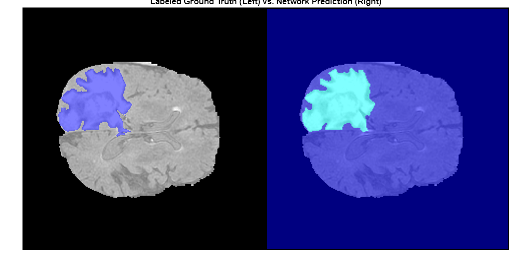
Display a montage showing the center slice of the ground truth and predicted labels along the depth direction.

zID = size(volTest,3)/2;
zSliceGT = labeloverlay(volTest(:,:,zID),volTestLabels(:,:,zID));
zSlicePred = labeloverlay(volTest(:,:,zID),predictedLabels(:,:,zID));

figure
montage({zSliceGT,zSlicePred},Size=[1 2],BorderSize=5) 
title("Labeled Ground Truth (Left) vs. Network Prediction (Right)")

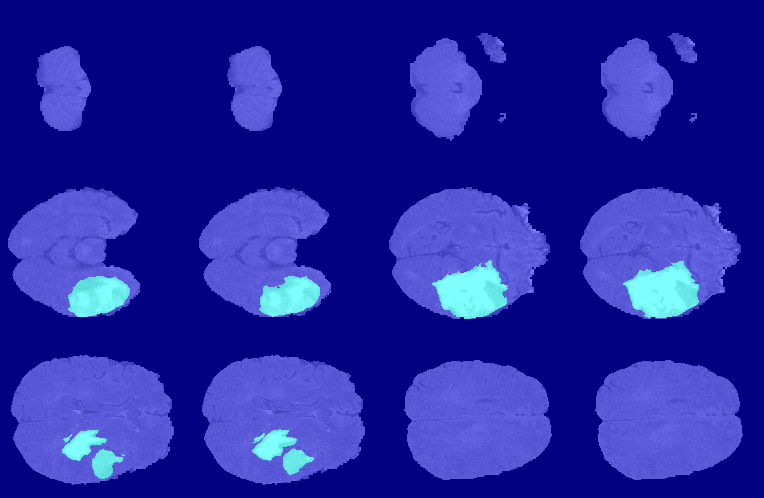
The following image shows the result of displaying slices sequentially across the one of the volumes. The labeled ground truth is on the left and the network prediction is on the right.

Download BraTS Data Set

If you do not want to download the training data set or train the network, then you can skip to the Evaluate Network Performance section of this example.

This example uses the BraTS data set [2]. The BraTS data set contains MRI scans of brain tumors, namely gliomas, which are the most common primary brain malignancies. The size of the data file is ~7 GB.

To download the BraTS data, go to the Medical Segmentation Decathlon website and click the "Download Data" link. Download the "Task01_BrainTumour.tar" file [3]. Unzip the TAR file into the directory specified by the imageDir variable. When unzipped successfully, imageDir will contain a directory named Task01_BrainTumour that has three subdirectories: imagesTr, imagesTs, and labelsTr.

The data set contains 750 4-D volumes, each representing a stack of 3-D images. Each 4-D volume has size 240-by-240-by-155-by-4, where the first three dimensions correspond to height, width, and depth of a 3-D volumetric image. The fourth dimension corresponds to different scan modalities. The data set is divided into 484 training volumes with voxel labels and 266 test volumes. The test volumes do not have labels so this example does not use the test data. Instead, the example splits the 484 training volumes into three independent sets that are used for training, validation, and testing.

Prepare Data for Training

To train the 3-D U-Net network more efficiently, preprocess the MRI data using the helper function preprocessBraTSDataset. This function is attached to the example as a supporting file. The helper function performs these operations:

Preprocessing the data can take about 30 minutes to complete.

sourceDataLoc = dataDir+filesep+"Task01_BrainTumour";
preprocessDataLoc = dataDir+filesep+"preprocessedDataset";
preprocessBraTSDataset(preprocessDataLoc,sourceDataLoc);

Create Random Patch Extraction Datastore for Training and Validation

Create an imageDatastore to store the 3-D image data. Because the MAT file format is a nonstandard image format, you must use a MAT file reader to enable reading the image data. You can use the helper MAT file reader, matRead. This function is attached to the example as a supporting file.

volLoc = fullfile(preprocessDataLoc,"imagesTr");
volds = imageDatastore(volLoc,FileExtensions=".mat",ReadFcn=@matRead);

Create a pixelLabelDatastore (Computer Vision Toolbox) to store the labels.

lblLoc = fullfile(preprocessDataLoc,"labelsTr");
classNames = ["background","tumor"];
pixelLabelID = [0 1];
pxds = pixelLabelDatastore(lblLoc,classNames,pixelLabelID, ...
    FileExtensions=".mat",ReadFcn=@matRead);

Create a randomPatchExtractionDatastore (Image Processing Toolbox) that extracts random patches from ground truth images and corresponding pixel label data. Specify a patch size of 132-by-132-by-132 voxels. Specify "PatchesPerImage" to extract 16 randomly positioned patches from each pair of volumes and labels during training. Specify a mini-batch size of 8.

patchSize = [132 132 132];
patchPerImage = 16;
miniBatchSize = 8;
patchds = randomPatchExtractionDatastore(volds,pxds,patchSize, ...
    PatchesPerImage=patchPerImage);
patchds.MiniBatchSize = miniBatchSize;

Create a randomPatchExtractionDatastore that extracts patches from the validation image and pixel label data. You can use validation data to evaluate whether the network is continuously learning, underfitting, or overfitting as time progresses.

volLocVal = fullfile(preprocessDataLoc,"imagesVal");
voldsVal = imageDatastore(volLocVal,FileExtensions=".mat", ...
    ReadFcn=@matRead);

lblLocVal = fullfile(preprocessDataLoc,"labelsVal");
pxdsVal = pixelLabelDatastore(lblLocVal,classNames,pixelLabelID, ...
    FileExtensions=".mat",ReadFcn=@matRead);

dsVal = randomPatchExtractionDatastore(voldsVal,pxdsVal,patchSize, ...
    PatchesPerImage=patchPerImage);
dsVal.MiniBatchSize = miniBatchSize;

Configure 3-D U-Net

This example uses the 3-D U-Net network [1]. In U-Net, the initial series of convolutional layers are interspersed with max pooling layers, successively decreasing the resolution of the input image. These layers are followed by a series of convolutional layers interspersed with upsampling operators, successively increasing the resolution of the input image. A batch normalization layer is introduced before each ReLU layer. The name U-Net comes from the fact that the network can be drawn with a symmetric shape like the letter U.

Create a default 3-D U-Net network by using the unetLayers (Computer Vision Toolbox) function. Specify two class segmentation. Also specify valid convolution padding to avoid border artifacts when using the overlap-tile strategy for prediction of the test volumes.

numChannels = 4;
inputPatchSize = [patchSize numChannels];
numClasses = 2;
[lgraph,outPatchSize] = unet3dLayers(inputPatchSize, ...
    numClasses,ConvolutionPadding="valid");

Augment the training and validation data by using the transform function with custom preprocessing operations specified by the helper function augmentAndCrop3dPatch. This function is attached to the example as a supporting file. The augmentAndCrop3dPatch function performs these operations:

dsTrain = transform(patchds, ...
    @(patchIn)augmentAndCrop3dPatch(patchIn,outPatchSize,"Training"));
dsVal = transform(dsVal, ...
    @(patchIn)augmentAndCrop3dPatch(patchIn,outPatchSize,"Validation"));

To better segment smaller tumor regions and reduce the influence of larger background regions, this example uses a dicePixelClassificationLayer (Computer Vision Toolbox). Replace the pixel classification layer with the Dice pixel classification layer.

outputLayer = dicePixelClassificationLayer(Name="Output");
lgraph = replaceLayer(lgraph,"Segmentation-Layer",outputLayer);

The data has already been normalized in the Preprocess Training and Validation Data section of this example. Data normalization in the image3dInputLayer is unnecessary, so replace the input layer with an input layer that does not have data normalization.

inputLayer = image3dInputLayer(inputPatchSize, ...
    Normalization="none",Name="ImageInputLayer");
lgraph = replaceLayer(lgraph,"ImageInputLayer",inputLayer);

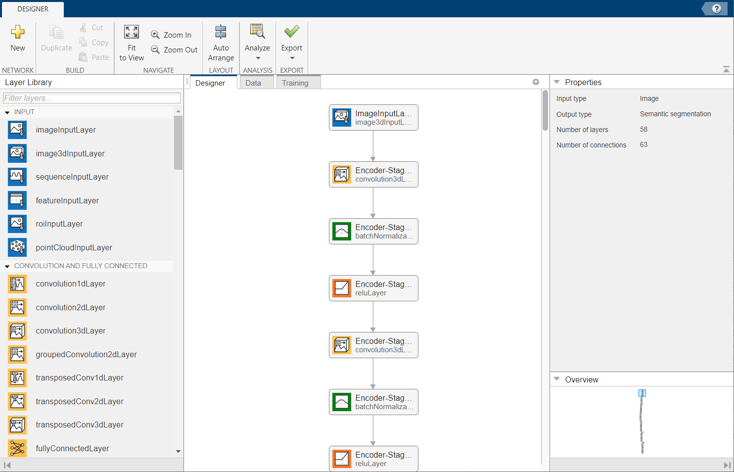
Alternatively, you can modify the 3-D U-Net network by using the Deep Network Designer app.

deepNetworkDesigner(lgraph)

Train 3-D U-Net

Specify Training Options

Train the network using the adam optimization solver. Specify the hyperparameter settings using the trainingOptions function. The initial learning rate is set to 5e-4 and gradually decreases over the span of training. You can experiment with the MiniBatchSize property based on your GPU memory. To maximize GPU memory utilization, favor large input patches over a large batch size. Note that batch normalization layers are less effective for smaller values of MiniBatchSize. Tune the initial learning rate based on the MiniBatchSize.

options = trainingOptions("adam", ...
    MaxEpochs=50, ...
    InitialLearnRate=5e-4, ...
    LearnRateSchedule="piecewise", ...
    LearnRateDropPeriod=5, ...
    LearnRateDropFactor=0.95, ...
    ValidationData=dsVal, ...
    ValidationFrequency=400, ...
    Plots="training-progress", ...
    Verbose=false, ...
    MiniBatchSize=miniBatchSize);

Train Network

By default, the example uses the downloaded pretrained 3-D U-Net network. The pretrained network enables you to perform semantic segmentation and evaluate the segmentation results without waiting for training to complete.

To train the network, set the doTraining variable in the following code to true. Train the network using the trainNetwork function.

Train on a GPU if one is available. Using a GPU requires Parallel Computing Toolbox™ and a CUDA® enabled NVIDIA® GPU. For more information, see GPU Computing Requirements (Parallel Computing Toolbox). Training takes about 30 hours on a multi-GPU system with 4 NVIDIA™ Titan Xp GPUs and can take even longer depending on your GPU hardware.

doTraining = false;
if doTraining
    [net,info] = trainNetwork(dsTrain,lgraph,options);
    modelDateTime = string(datetime("now",Format="yyyy-MM-dd-HH-mm-ss"));
    save("trained3DUNet-"+modelDateTime+".mat","net");
end

Evaluate 3-D U-Net

Select the source of test data that contains ground truth volumes and labels for testing. If you keep the useFullTestSet variable in the following code as false, then the example uses five sample volumes for testing. If you set the useFullTestSet variable to true, then the example uses 55 test images selected from the full data set.

useFullTestSet = false;
if useFullTestSet
    volLocTest = fullfile(preprocessDataLoc,"imagesTest");
    lblLocTest = fullfile(preprocessDataLoc,"labelsTest");
else
    volLocTest = fullfile(testDir,"imagesTest");
    lblLocTest = fullfile(testDir,"labelsTest");
end

The voldsTest variable stores the ground truth test images. The pxdsTest variable stores the ground truth labels.

voldsTest = imageDatastore(volLocTest,FileExtensions=".mat", ...
    ReadFcn=@matRead);
pxdsTest = pixelLabelDatastore(lblLocTest,classNames,pixelLabelID, ...
    FileExtensions=".mat",ReadFcn=@matRead);

For each test volume, process each block using the apply (Image Processing Toolbox) function. The apply function performs the operations specified by the helper function calculateBlockMetrics, which is defined at the end of this example. The calculateBlockMetrics function performs semantic segmentation of each block and calculates the confusion matrix between the predicted and ground truth labels.

imageIdx = 1;
datasetConfMat = table;
while hasdata(voldsTest)

    % Read volume and label data
    vol = read(voldsTest);
    volLabels = read(pxdsTest);

    % Create blockedImage for volume and label data
    testVolume = blockedImage(vol);
    testLabels = blockedImage(volLabels{1});

    % Calculate block metrics
    blockConfMatOneImage = apply(testVolume, ...
        @(block,labeledBlock) ...
            calculateBlockMetrics(block,labeledBlock,net), ...
        ExtraImages=testLabels, ...
        PadPartialBlocks=true, ...
        BlockSize=blockSize, ...
        BorderSize=borderSize, ...
        UseParallel=false);

    % Read all the block results of an image and update the image number
    blockConfMatOneImageDS = blockedImageDatastore(blockConfMatOneImage);
    blockConfMat = readall(blockConfMatOneImageDS);
    blockConfMat = struct2table([blockConfMat{:}]);
    blockConfMat.ImageNumber = imageIdx.*ones(height(blockConfMat),1);
    datasetConfMat = [datasetConfMat;blockConfMat];

    imageIdx = imageIdx + 1;
end

Evaluate the data set metrics and block metrics for the segmentation using the evaluateSemanticSegmentation (Computer Vision Toolbox) function.

[metrics,blockMetrics] = evaluateSemanticSegmentation( ...
    datasetConfMat,classNames,Metrics="all");

Evaluating semantic segmentation results
----------------------------------------
* Selected metrics: global accuracy, class accuracy, IoU, weighted IoU.
* Processed 5 images.
* Finalizing... Done.
* Data set metrics:

    GlobalAccuracy    MeanAccuracy    MeanIoU    WeightedIoU
    ______________    ____________    _______    ___________

       0.99902          0.97955       0.95978      0.99808  

Display the Jaccard score calculated for each image.

metrics.ImageMetrics.MeanIoU

ans = 5×1

    0.9613
    0.9570
    0.9551
    0.9656
    0.9594

Supporting Function

The calculateBlockMetrics helper function performs semantic segmentation of a block and calculates the confusion matrix between the predicted and ground truth labels. The function returns a structure with fields containing the confusion matrix and metadata about the block. You can use the structure with the evaluateSemanticSegmentation function to calculate metrics and aggregate block-based results.

function blockMetrics = calculateBlockMetrics(bstruct,gtBlockLabels,net)

% Segment block
predBlockLabels = semanticseg(bstruct.Data,net);

% Trim away border region from gtBlockLabels 
blockStart = bstruct.BorderSize + 1;
blockEnd = blockStart + bstruct.BlockSize - 1;
gtBlockLabels = gtBlockLabels( ...
    blockStart(1):blockEnd(1), ...
    blockStart(2):blockEnd(2), ...
    blockStart(3):blockEnd(3));

% Evaluate segmentation results against ground truth
confusionMat = segmentationConfusionMatrix(predBlockLabels,gtBlockLabels);

% blockMetrics is a struct with confusion matrices, image number,
% and block information. 
blockMetrics.ConfusionMatrix = confusionMat;
blockMetrics.ImageNumber = bstruct.ImageNumber;
blockInfo.Start = bstruct.Start;
blockInfo.End = bstruct.End;
blockMetrics.BlockInfo = blockInfo;

end

References

[1] Çiçek, Ö., A. Abdulkadir, S. S. Lienkamp, T. Brox, and O. Ronneberger. "3D U-Net: Learning Dense Volumetric Segmentation from Sparse Annotation." In Proceedings of the International Conference on Medical Image Computing and Computer-Assisted Intervention - MICCAI 2016. Athens, Greece, Oct. 2016, pp. 424-432.

[2] Isensee, F., P. Kickingereder, W. Wick, M. Bendszus, and K. H. Maier-Hein. "Brain Tumor Segmentation and Radiomics Survival Prediction: Contribution to the BRATS 2017 Challenge." In Proceedings of BrainLes: International MICCAI Brainlesion Workshop. Quebec City, Canada, Sept. 2017, pp. 287-297.

[3] "Brain Tumours". Medical Segmentation Decathlon. http://medicaldecathlon.com/

The BraTS dataset is provided by Medical Segmentation Decathlon under the CC-BY-SA 4.0 license. All warranties and representations are disclaimed; see the license for details. bat365® has modified the data set linked in the Download BraTS Sample Data section of this example. The modified sample data set has been cropped to a region containing primarily the brain and tumor and each channel has been normalized independently by subtracting the mean and dividing by the standard deviation of the cropped brain region.

[4] Sudre, C. H., W. Li, T. Vercauteren, S. Ourselin, and M. J. Cardoso. "Generalised Dice Overlap as a Deep Learning Loss Function for Highly Unbalanced Segmentations." Deep Learning in Medical Image Analysis and Multimodal Learning for Clinical Decision Support: Third International Workshop. Quebec City, Canada, Sept. 2017, pp. 240-248.

[5] Ronneberger, O., P. Fischer, and T. Brox. "U-Net:Convolutional Networks for Biomedical Image Segmentation." In Proceedings of the International Conference on Medical Image Computing and Computer-Assisted Intervention - MICCAI 2015. Munich, Germany, Oct. 2015, pp. 234-241. Available at arXiv:1505.04597.