bat365 Homepage

Multilabel Text Classification Using Deep Learning

This example uses:

This example shows how to classify text data that has multiple independent labels.

For classification tasks where there can be multiple independent labels for each observation—for example, tags on an scientific article—you can train a deep learning model to predict probabilities for each independent class. To enable a network to learn multilabel classification targets, you can optimize the loss of each class independently using binary cross-entropy loss.

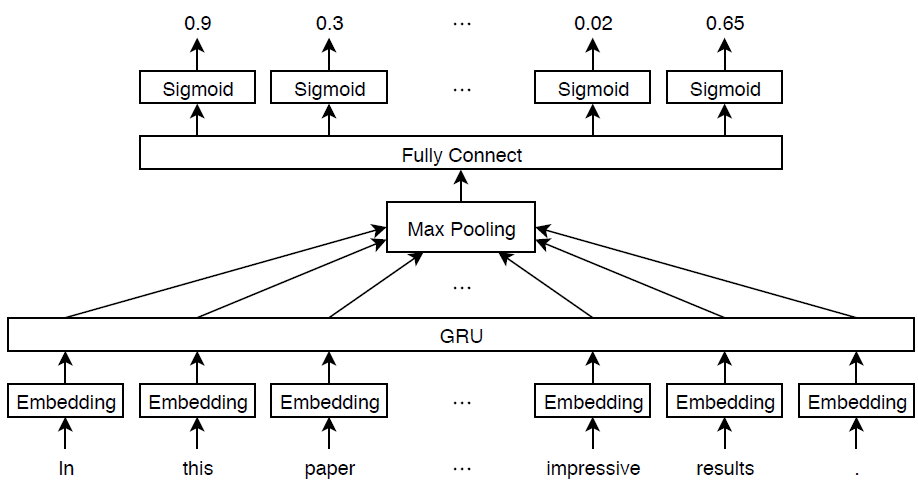
This example defines a deep learning model that classifies subject areas given the abstracts of mathematical papers collected using the arXiv API [1]. The model consists of a word embedding and GRU, max pooling operation, fully connected, and sigmoid operations.

To measure the performance of multilabel classification, you can use the labeling F-score [2]. The labeling F-score evaluates multilabel classification by focusing on per-text classification with partial matches. The measure is the normalized proportion of matching labels against the total number of true and predicted labels.

This example defines the following model:

A word embedding that maps a sequence of words to a sequence of numeric vectors.
A GRU operation that learns dependencies between the embedding vectors.
A max pooling operation that reduces a sequence of feature vectors to a single feature vector.
A fully connected layer that maps the features to the binary outputs.
A sigmoid operation for learning the binary cross entropy loss between the outputs and the target labels.

This diagram shows a piece of text propagating through the model architecture and outputting a vector of probabilities. The probabilities are independent, so they need not sum to one.

Import Text Data

Import a set of abstracts and category labels from math papers using the arXiv API. Specify the number of records to import using the importSize variable.

importSize = 50000;

Create a URL that queries records with set "math" and metadata prefix "arXiv".

url = "https://export.arxiv.org/oai2?verb=ListRecords" + ...
    "&set=math" + ...
    "&metadataPrefix=arXiv";

Extract the abstract text, category labels, and the resumption token returned by the query URL using the parseArXivRecords function which is attached to this example as a supporting file. To access this file, open this example as a live script. Note that the arXiv API is rate limited and requires waiting between multiple requests.

[textData,labelsAll,resumptionToken] = parseArXivRecords(url);

Iteratively import more chunks of records until the required amount is reached, or there are no more records. To continue importing records from where you left off, use the resumption token from the previous result in the query URL. To adhere to the rate limits imposed by the arXiv API, add a delay of 20 seconds before each query using the pause function.

while numel(textData) < importSize
    
    if resumptionToken == ""
        break
    end
    
    url = "https://export.arxiv.org/oai2?verb=ListRecords" + ...
        "&resumptionToken=" + resumptionToken;
    
    pause(20)
    [textDataNew,labelsNew,resumptionToken] = parseArXivRecords(url);
    
    textData = [textData; textDataNew];
    labelsAll = [labelsAll; labelsNew];
end

Preprocess Text Data

Tokenize and preprocess the text data using the preprocessText function, listed at the end of the example.

documentsAll = preprocessText(textData);
documentsAll(1:5)

ans = 
  5×1 tokenizedDocument:

    72 tokens: describe new algorithm $(k,\ell)$ pebble game color obtain characterization family $(k,\ell)$ sparse graph algorithmic solution family problem concerning tree decomposition graph special instance sparse graph appear rigidity theory receive increase attention recent year particular colored pebble generalize strengthen previous result lee streinu give new proof tuttenashwilliams characterization arboricity present new decomposition certify sparsity base $(k,\ell)$ pebble game color work expose connection pebble game algorithm previous sparse graph algorithm gabow gabow westermann hendrickson
    22 tokens: show determinant stirling cycle number count unlabeled acyclic singlesource automaton proof involve bijection automaton certain marked lattice path signreversing involution evaluate determinant
    18 tokens: paper show compute $\lambda_{\alpha}$ norm alpha dyadic grid result consequence description hardy space $h^p(r^n)$ term dyadic special atom
    62 tokens: partial cube isometric subgraphs hypercubes structure graph define mean semicubes djokovi winklers relation play important role theory partial cube structure employ paper characterize bipartite graph partial cube arbitrary dimension new characterization establish new proof know result give operation cartesian product paste expansion contraction process utilize paper construct new partial cube old particular isometric lattice dimension finite partial cube obtain mean operation calculate
    29 tokens: paper present algorithm compute hecke eigensystems hilbertsiegel cusp form real quadratic field narrow class number give illustrative example quadratic field $\q(\sqrt{5})$ example identify hilbertsiegel eigenforms possible lift hilbert eigenforms

Remove labels that do not belong to the "math" set.

for i = 1:numel(labelsAll)
    labelsAll{i} = labelsAll{i}(startsWith(labelsAll{i},"math."));
end

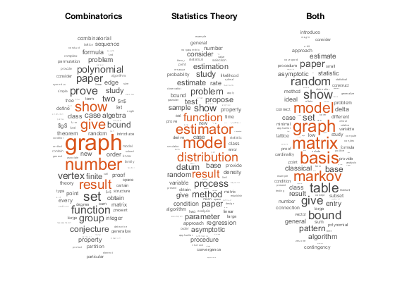
Visualize some of the classes in a word cloud. Find the documents corresponding to the following:

Abstracts tagged with "Combinatorics" and not tagged with "Statistics Theory"
Abstracts tagged with "Statistics Theory" and not tagged with "Combinatorics"
Abstracts tagged with both "Combinatorics" and "Statistics Theory"

Find the document indices for each of the groups using the ismember function.

idxCO = cellfun(@(lbls) ismember("math.CO",lbls) && ~ismember("math.ST",lbls),labelsAll);
idxST = cellfun(@(lbls) ismember("math.ST",lbls) && ~ismember("math.CO",lbls),labelsAll);
idxCOST = cellfun(@(lbls) ismember("math.CO",lbls) && ismember("math.ST",lbls),labelsAll);

Visualize the documents for each group in a word cloud.

figure
subplot(1,3,1)
wordcloud(documentsAll(idxCO));
title("Combinatorics")

subplot(1,3,2)
wordcloud(documentsAll(idxST));
title("Statistics Theory")

subplot(1,3,3)
wordcloud(documentsAll(idxCOST));
title("Both")

View the number of classes.

classNames = unique(cat(1,labelsAll{:}));
numClasses = numel(classNames)

numClasses = 32

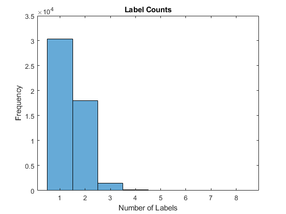
Visualize the number of per-document labels using a histogram.

labelCounts = cellfun(@numel,labelsAll);
figure
histogram(labelCounts)
xlabel("Number of Labels")
ylabel("Frequency")
title("Label Counts")

Prepare Text Data for Deep Learning

Partition the data into training and validation partitions using the cvpartition function. Hold out 10% of the data for validation by setting the HoldOut option to 0.1.

cvp = cvpartition(numel(documentsAll),HoldOut=0.1);
documentsTrain = documentsAll(training(cvp));
documentsValidation = documentsAll(test(cvp));

labelsTrain = labelsAll(training(cvp));
labelsValidation = labelsAll(test(cvp));

Create a word encoding object that encodes the training documents as sequences of word indices. Specify a vocabulary of the 5000 words by setting the Order option to "frequency", and the MaxNumWords option to 5000.

enc = wordEncoding(documentsTrain,Order="frequency",MaxNumWords=5000)

enc = 
  wordEncoding with properties:

      NumWords: 5000
    Vocabulary: [1×5000 string]

To improve training, use the following techniques:

When training, truncate the documents to a length that reduces the amount of padding used and does not does discard too much data.
Train for one epoch with the documents sorted by length in ascending order, then shuffle the data each epoch. This technique is known as sortagrad.

To choose a sequence length for truncation, visualize the document lengths in a histogram and choose a value that captures most of the data.

documentLengths = doclength(documentsTrain);

figure
histogram(documentLengths)
xlabel("Document Length")
ylabel("Frequency")
title("Document Lengths")

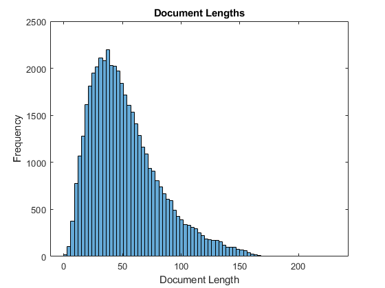
Most of the training documents have fewer than 175 tokens. Use 175 tokens as the target length for truncation and padding.

maxSequenceLength = 175;

To use the sortagrad technique, sort the documents by length in ascending order.

[~,idx] = sort(documentLengths);
documentsTrain = documentsTrain(idx);
labelsTrain = labelsTrain(idx);

Define and Initialize Model Parameters

Define the parameters for each of the operations and include them in a struct. Use the format parameters.OperationName.ParameterName, where parameters is the struct, OperationName is the name of the operation (for example "fc"), and ParameterName is the name of the parameter (for example, "Weights").

Create a struct parameters containing the model parameters. Initialize the bias with zeros. Use the following weight initializers for the operations:

For the embedding, initialize the weights using the initializeGaussian function.
For the GRU operation, initialize the weights and bias using the initializeGlorot and initializeZeros functions, respectively.
For the fully connect operation, initialize the weights and bias using the initializeGaussian and initializeZeros functions, respectively.

The initialization functions initializeGlorot, initializeGaussian, and initializeZeros are attached to the example as supporting files. To access these functions, open the example as a live script.

Initialize the learnable parameters for the embedding.

embeddingDimension = 300;
numHiddenUnits = 250;
inputSize = enc.NumWords + 1;

parameters = struct;

sz = [embeddingDimension inputSize];
mu = 0;
sigma = 0.01;
parameters.emb.Weights = initializeGaussian(sz,mu,sigma);

Initialize the learnable parameters for the GRU operation using.

sz = [3*numHiddenUnits embeddingDimension];
numOut = 3*numHiddenUnits;
numIn = embeddingDimension;
parameters.gru.InputWeights = initializeGlorot(sz,numOut,numIn);

sz = [3*numHiddenUnits numHiddenUnits];
numOut = 3*numHiddenUnits;
numIn = numHiddenUnits;
parameters.gru.RecurrentWeights = initializeGlorot(sz,numOut,numIn);

sz = [3*numHiddenUnits 1];
parameters.gru.Bias = initializeZeros(sz);

Initialize the learnable parameters for the fully connect operation.

sz = [numClasses numHiddenUnits];
mu = 0;
sigma = 0.01;
parameters.fc.Weights = initializeGaussian(sz,mu,sigma);

sz = [numClasses 1];
parameters.fc.Bias = initializeZeros(sz);

View the parameters struct.

parameters

parameters = struct with fields:
    emb: [1×1 struct]
    gru: [1×1 struct]
     fc: [1×1 struct]

View the parameters for the GRU operation.

parameters.gru

ans = struct with fields:
        InputWeights: [750×300 dlarray]
    RecurrentWeights: [750×250 dlarray]
                Bias: [750×1 dlarray]

Define Model Function

Create the function model, listed at the end of the example, which computes the outputs of the deep learning model described earlier. The function model takes as input the input data and the model parameters. The network outputs the predictions for the labels.

Define Model Loss Function

Create the function modelLoss, listed at the end of the example, which takes as input a mini-batch of input data and the corresponding targets, and returns the loss, the gradients of the loss with respect to the learnable parameters, and the network outputs.

Specify Training Options

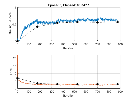
Train for 5 epochs with a mini-batch size of 256.

numEpochs = 5;
miniBatchSize = 256;

Train using the Adam optimizer, with a learning rate of 0.01, and specify gradient decay and squared gradient decay factors of 0.5 and 0.999, respectively.

learnRate = 0.01;
gradientDecayFactor = 0.5;
squaredGradientDecayFactor = 0.999;

Clip the gradients with a threshold of 1 using $L_{2}$ norm gradient clipping.

gradientThreshold = 1;

To convert a vector of probabilities to labels, use the labels with probabilities higher than a specified threshold. Specify a label threshold of 0.5.

labelThreshold = 0.5;

Validate the network every epoch.

numObservationsTrain = numel(documentsTrain);
numIterationsPerEpoch = floor(numObservationsTrain/miniBatchSize);
validationFrequency = numIterationsPerEpoch;

Train Model

Initialize the training progress plot. Create animated lines for the F-score and the loss.

figure
C = colororder;

subplot(2,1,1)
lineFScoreTrain = animatedline(Color=C(1,:));
lineFScoreValidation = animatedline( ...
    LineStyle="--", ...
    Marker="o", ...
    MarkerFaceColor="black");
ylim([0 1])
xlabel("Iteration")
ylabel("Labeling F-Score")
grid on

subplot(2,1,2)
lineLossTrain = animatedline(Color=C(2,:));
lineLossValidation = animatedline( ...
    LineStyle="--", ...
    Marker="o", ...
    MarkerFaceColor="black");
ylim([0 inf])
xlabel("Iteration")
ylabel("Loss")
grid on

Initialize parameters for the Adam optimizer.

trailingAvg = [];
trailingAvgSq = [];

Prepare the validation data. Create a one-hot encoded matrix where non-zero entries correspond to the labels of each observation.

numObservationsValidation = numel(documentsValidation);
TValidation = zeros(numClasses, numObservationsValidation,"single");
for i = 1:numObservationsValidation
    [~,idx] = ismember(labelsValidation{i},classNames);
    TValidation(idx,i) = 1;
end

Train the model using a custom training loop.

For each epoch, loop over mini-batches of data. At the end of each epoch, shuffle the data. At the end of each iteration, update the training progress plot.

For each mini-batch:

Convert the documents to sequences of word indices and convert the labels to dummy variables.
Convert the sequences to dlarray objects with underlying type single and specify the dimension labels "BTC" (batch, time, channel).
Train on a GPU if one is available. This requires Parallel Computing Toolbox™. Using a GPU requires Parallel Computing Toolbox™ and a supported GPU device. For information on supported devices, see GPU Computing Requirements (Parallel Computing Toolbox).
For GPU training, convert to gpuArray objects.
Evaluate the model loss and gradients using dlfeval and the modelLoss function.
Clip the gradients.
Update the network parameters using the adamupdate function.
If necessary, validate the network using the modelPredictions function, listed at the end of the example.
Update the training plot.

iteration = 0;
start = tic;

% Loop over epochs.
for epoch = 1:numEpochs
    
    % Loop over mini-batches.
    for i = 1:numIterationsPerEpoch
        iteration = iteration + 1;
        idx = (i-1)*miniBatchSize+1:i*miniBatchSize;
        
        % Read mini-batch of data and convert the labels to dummy
        % variables.
        documents = documentsTrain(idx);
        labels = labelsTrain(idx);
        
        % Convert documents to sequences.
        len = min(maxSequenceLength,max(doclength(documents)));
        X = doc2sequence(enc,documents, ...
            PaddingValue=inputSize, ...
            Length=len);
        X = cat(1,X{:});
        
        % Dummify labels.
        T = zeros(numClasses,miniBatchSize,"single");
        for j = 1:miniBatchSize
            [~,idx2] = ismember(labels{j},classNames);
            T(idx2,j) = 1;
        end
        
        % Convert mini-batch of data to dlarray.
        X = dlarray(X,"BTC");
        
        % If training on a GPU, then convert data to gpuArray.
        if canUseGPU
            X = gpuArray(X);
        end
        
        % Evaluate the model loss, gradients, and predictions using dlfeval and the
        % modelLoss function.
        [loss,gradients,Y] = dlfeval(@modelLoss,X,T,parameters);
        
        % Gradient clipping.
        gradients = dlupdate(@(g) thresholdL2Norm(g,gradientThreshold),gradients);
        
        % Update the network parameters using the Adam optimizer.
        [parameters,trailingAvg,trailingAvgSq] = adamupdate(parameters,gradients, ...
            trailingAvg,trailingAvgSq,iteration,learnRate, ...
            gradientDecayFactor,squaredGradientDecayFactor);

        % Display the training progress.
        subplot(2,1,1)
        D = duration(0,0,toc(start),Format="hh:mm:ss");
        title("Epoch: " + epoch + ", Elapsed: " + string(D))

        % Loss.
        loss = double(loss);
        addpoints(lineLossTrain,iteration,loss)

        % Labeling F-score.
        Y = Y > labelThreshold;
        score = labelingFScore(Y,T);
        addpoints(lineFScoreTrain,iteration,double(gather(score)))

        drawnow

        % Display validation metrics.
        if iteration == 1 || mod(iteration,validationFrequency) == 0
            YValidation = modelPredictions(parameters,enc,documentsValidation,miniBatchSize,maxSequenceLength);

            % Loss.
            lossValidation = crossentropy(YValidation,TValidation, ...
                ClassificationMode="multilabel", ...
                DataFormat="CB");
            lossValidation = double(lossValidation);
            addpoints(lineLossValidation,iteration,lossValidation)

            % Labeling F-score.
            YValidation = YValidation > labelThreshold;
            score = labelingFScore(YValidation,TValidation);
            score = double(score);
            addpoints(lineFScoreValidation,iteration,score)

            drawnow
        end
    end
    
    % Shuffle data.
    idx = randperm(numObservationsTrain);
    documentsTrain = documentsTrain(idx);
    labelsTrain = labelsTrain(idx);
end

Test Model

To make predictions on a new set of data, use the modelPredictions function, listed at the end of the example. The modelPredictions function takes as input the model parameters, a word encoding, and an array of tokenized documents, and outputs the model predictions corresponding to the specified mini-batch size and the maximum sequence length.

YValidation = modelPredictions(parameters,enc,documentsValidation,miniBatchSize,maxSequenceLength);

To evaluate the performance, calculate the labeling F-score using the labelingFScore function, listed at the end of the example. The labeling F-score evaluates multilabel classification by focusing on per-text classification with partial matches. To convert the network outputs to an array of labels, find the labels with scores higher than the specified label threshold.

score = labelingFScore(YValidation > labelThreshold,TValidation)

score = single
    0.5663

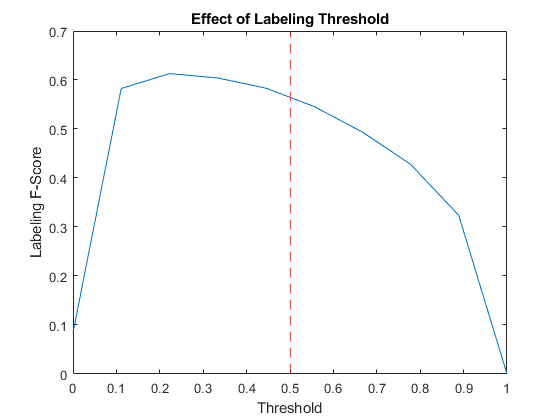
View the effect of the labeling threshold on the labeling F-score by trying a range of values for the threshold and comparing the results.

thr = linspace(0,1,10);
score = zeros(size(thr));
for i = 1:numel(thr)
    YPredValidationThr = YValidation >= thr(i);
    score(i) = labelingFScore(YPredValidationThr,TValidation);
end

figure
plot(thr,score)
xline(labelThreshold,"r--");
xlabel("Threshold")
ylabel("Labeling F-Score")
title("Effect of Labeling Threshold")

Visualize Predictions

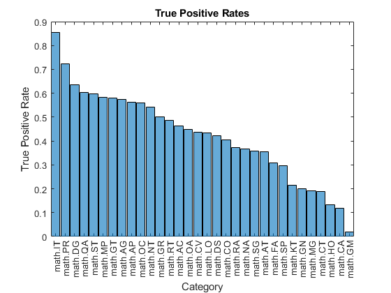
To visualize the correct predictions of the classifier, calculate the numbers of true positives. A true positive is an instance of a classifier correctly predicting a particular class for an observation.

Y = YValidation > labelThreshold;
T = TValidation;

numTruePositives = sum(T & Y,2);

numObservationsPerClass = sum(T,2);
truePositiveRates = numTruePositives ./ numObservationsPerClass;

Visualize the numbers of true positives for each class in a histogram.

figure
truePositiveRates = extractdata(truePositiveRates);
[~,idx] = sort(truePositiveRates,"descend");
histogram(Categories=classNames(idx),BinCounts=truePositiveRates(idx))
xlabel("Category")
ylabel("True Positive Rate")
title("True Positive Rates")

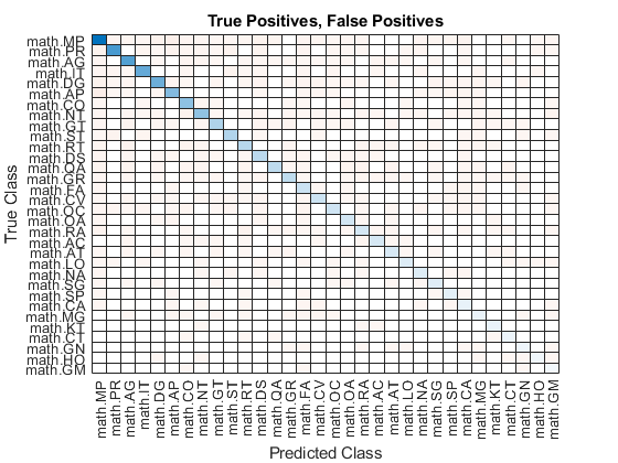
Visualize the instances where the classifier predicts incorrectly by showing the distribution of true positives, false positives, and false negatives. A false positive is an instance of a classifier assigning a particular incorrect class to an observation. A false negative is an instance of a classifier failing to assign a particular correct class to an observation.

Create a confusion matrix showing the true positive, false positive, and false negative counts:

For each class, display the true positive counts on the diagonal.
For each pair of classes (i,j), display the number of instances of a false positive for j when the instance is also a false negative for i.

That is, the confusion matrix with elements given by:

${TPFN}_{i j} = {\begin{array}{c} numTruePositives (i), & if i = j \\ numFalsePositives (j | i is a false negative), & if i \neq j \end{array}$

Calculate the false negatives and false positives.

falseNegatives = T & ~Y;
falsePositives = ~T & Y;

Calculate the off-diagonal elements.

falseNegatives = permute(falseNegatives,[3 2 1]);
numConditionalFalsePositives = sum(falseNegatives & falsePositives, 2);
numConditionalFalsePositives = squeeze(numConditionalFalsePositives);

tpfnMatrix = numConditionalFalsePositives;

Set the diagonal elements to the true positive counts.

idxDiagonal = 1:numClasses+1:numClasses^2;
tpfnMatrix(idxDiagonal) = numTruePositives;

Visualize the true positive and false positive counts in a confusion matrix using the confusionchart function and sort the matrix such that the elements on the diagonal are in descending order.

figure
tpfnMatrix = extractdata(tpfnMatrix);
cm = confusionchart(tpfnMatrix,classNames);
sortClasses(cm,"descending-diagonal");
title("True Positives, False Positives")

To view the matrix in more detail, open this example as a live script and open the figure in a new window.

Preprocess Text Function

The preprocessText function tokenizes and preprocesses the input text data using the following steps:

Tokenize the text using the tokenizedDocument function. Extract mathematical equations as a single token using the RegularExpressions option by specifying the regular expression "\$.*?\$", which captures text appearing between two "$" symbols.
Erase the punctuation using the erasePunctuation function.
Convert the text to lowercase using the lower function.
Remove the stop words using the removeStopWords function.
Lemmatize the text using the normalizeWords function with the Style option set to "lemma".

function documents = preprocessText(textData)

% Tokenize the text.
regularExpressions = table;
regularExpressions.Pattern = "\$.*?\$";
regularExpressions.Type = "equation";

documents = tokenizedDocument(textData,RegularExpressions=regularExpressions);

% Erase punctuation.
documents = erasePunctuation(documents);

% Convert to lowercase.
documents = lower(documents);

% Lemmatize.
documents = addPartOfSpeechDetails(documents);
documents = normalizeWords(documents,Style="lemma");

% Remove stop words.
documents = removeStopWords(documents);

% Remove short words.
documents = removeShortWords(documents,2);

end

Model Function

The function model takes as input the input data X and the model parameters parameters, and returns the predictions for the labels.

function Y = model(X,parameters)

% Embedding
weights = parameters.emb.Weights;
X = embed(X,weights);

% GRU
inputWeights = parameters.gru.InputWeights;
recurrentWeights = parameters.gru.RecurrentWeights;
bias = parameters.gru.Bias;

numHiddenUnits = size(inputWeights,1)/3;
hiddenState = dlarray(zeros([numHiddenUnits 1]));

Y = gru(X,hiddenState,inputWeights,recurrentWeights,bias);

% Max pooling along time dimension
Y = max(Y,[],3);

% Fully connect
weights = parameters.fc.Weights;
bias = parameters.fc.Bias;
Y = fullyconnect(Y,weights,bias);

% Sigmoid
Y = sigmoid(Y);

end

Model Loss Function

The modelLoss function takes as input a mini-batch of input data X with corresponding targets T containing the labels and returns the loss, the gradients of the loss with respect to the learnable parameters, and the network outputs.

function [loss,gradients,Y] = modelLoss(X,T,parameters)

Y = model(X,parameters);

loss = crossentropy(Y,T,ClassificationMode="multilabel");

gradients = dlgradient(loss,parameters);

end

Model Predictions Function

The modelPredictions function takes as input the model parameters, a word encoding, an array of tokenized documents, a mini-batch size, and a maximum sequence length, and returns the model predictions by iterating over mini-batches of the specified size.

function Y = modelPredictions(parameters,enc,documents,miniBatchSize,maxSequenceLength)

inputSize = enc.NumWords + 1;

numObservations = numel(documents);
numIterations = ceil(numObservations / miniBatchSize);

numFeatures = size(parameters.fc.Weights,1);
Y = zeros(numFeatures,numObservations,"like",parameters.fc.Weights);

for i = 1:numIterations
    
    idx = (i-1)*miniBatchSize+1:min(i*miniBatchSize,numObservations);
    
    len = min(maxSequenceLength,max(doclength(documents(idx))));
    X = doc2sequence(enc,documents(idx), ...
        PaddingValue=inputSize, ...
        Length=len);
    X = cat(1,X{:});
    
    X = dlarray(X,"BTC");
    
    Y(:,idx) = model(X,parameters);
end

end

Labeling F-Score Function

The labeling F-score function [2] evaluates multilabel classification by focusing on per-text classification with partial matches. The measure is the normalized proportion of matching labels against the total number of true and predicted labels given by

$\frac{1}{N} \sum_{n = 1}^{N} (\frac{2 \sum_{c = 1}^{C} Y_{n c} T_{n c}}{\sum_{c = 1}^{C} (Y_{n c} + T_{n c})}),$

where N and C correspond to the number of observations and classes, respectively, and Y and T correspond to the predictions and targets, respectively.

function score = labelingFScore(Y,T)

numObservations = size(T,2);

scores = (2 * sum(Y .* T)) ./ sum(Y + T);
score = sum(scores) / numObservations;

end

Gradient Clipping Function

The thresholdL2Norm function scales the input gradients so that their $L_{2}$ norm values equal the specified gradient threshold when the $L_{2}$ norm value of the gradient of a learnable parameter is larger than the specified threshold.

function gradients = thresholdL2Norm(gradients,gradientThreshold)

gradientNorm = sqrt(sum(gradients(:).^2));
if gradientNorm > gradientThreshold
    gradients = gradients * (gradientThreshold / gradientNorm);
end

end

References

arXiv. "arXiv API." Accessed January 15, 2020. https://arxiv.org/help/api
Sokolova, Marina, and Guy Lapalme. "A Systematic Analysis of Performance Measures for Classification Tasks." Information Processing & Management 45, no. 4 (2009): 427–437.