Fit Smooth Surfaces to Investigate Fuel Efficiency
This example shows how to use Curve Fitting Toolbox™ to fit a response surface to some automotive data to investigate fuel efficiency.
The toolbox provides sample data generated from a GTPOWER predictive combustion engine model. The model emulates a naturally aspirated spark-ignition, 2-liter, inline 4-cylinder engine. You can fit smooth lowess surfaces to this data to find minimum fuel consumption.
The data set includes the required variables to model response surfaces:
Speed is in revolutions per minute (rpm) units.
Load is the normalized cylinder air mass (the ratio of cylinder aircharge to maximum naturally aspirated cylinder aircharge at standard temperature and pressure).
BSFC is the brake-specific fuel consumption in g/KWh. That is, the energy flow in, divided by mechanical power out (fuel efficiency).
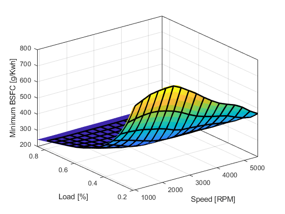
The aim is to model a response surface to find the minimum BSFC as a function of speed and load. You can use this surface as a table, included as part of a hybrid vehicle optimization algorithm combining the use of a motor and your engine. To operate the engine as fuel efficiently as possible, the table must operate the engine near the bottom of the BSFC bowl.
Load and Preprocess Data
Load the data from the XLS spreadsheet. Use the 'basic' command option for non-Windows® platforms.
Create a variable n that has all the numeric data in one array.
n = xlsread( 'Engine_Data_SI_NA_2L_I4.xls', 'SI NA 2L I4', '', 'basic' );
Extract from the variable n the columns of interest.
SPEED = n(:,2);
LOAD_CMD = n(:,3);
LOAD = n(:,8);
BSFC = n(:,22);
Process the data before fitting, to pick out the minimum BSFC values from each sweep. The data points are organized in sweeps on speed/load.
Get a list of the speed/load sites:
SL = unique( [SPEED, LOAD_CMD], 'rows' );
nRuns = size( SL, 1 );
For each speed/load site, find the data at the site and extract the actual measured load and the minimum BSFC.
minBSFC  = zeros( nRuns, 1 );
Load     = zeros( nRuns, 1 );
Speed    = zeros( nRuns, 1 );
for i = 1:nRuns
    idx = SPEED == SL(i,1) & LOAD_CMD == SL(i,2);

    minBSFC(i) = min(  BSFC(idx) );
    Load(i)    = mean( LOAD(idx) );
    Speed(i)   = mean( SPEED(idx) );
end
Fit a Surface
Fit a surface of fuel efficiency to the preprocessed data.
f1 = fit( [Speed, Load], minBSFC, 'Lowess', 'Normalize', 'on' )
     Locally weighted smoothing linear regression:
       f1(x,y) = lowess (linear) smoothing regression computed from p
       where x is normalized by mean 3407 and std 1214
       and where y is normalized by mean 0.5173 and std 0.1766
     Coefficients:
       p = coefficient structure
Plot Fit
plot( f1, [Speed, Load], minBSFC );
xlabel( 'Speed [RPM]' );
ylabel( 'Load [%]' );
zlabel( 'Minimum BSFC [g/Kwh]' );
Remove Problem Points
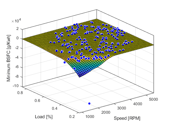
Review the resulting plot.
There are points where BSFC is negative because this data is generated by an engine simulation.
Remove those problem data points by keeping points in the range [0, Inf].
out = excludedata( Speed, minBSFC, 'Range', [0, Inf] );
f2 = fit( [Speed, Load], minBSFC, 'Lowess', ...
    'Normalize', 'on', 'Exclude', out )
     Locally weighted smoothing linear regression:
       f2(x,y) = lowess (linear) smoothing regression computed from p
       where x is normalized by mean 3443 and std 1187
       and where y is normalized by mean 0.521 and std 0.175
     Coefficients:
       p = coefficient structure
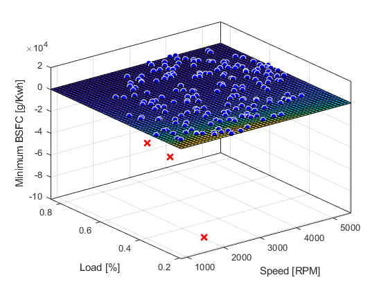
Plot the new fit. Note that the excluded points are plotted as red crosses.
plot( f2, [Speed, Load], minBSFC, 'Exclude', out );
xlabel( 'Speed [RPM]' );
ylabel( 'Load [%]' );
zlabel( 'Minimum BSFC [g/Kwh]' );
Zoom In
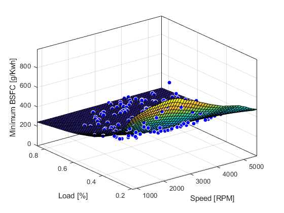
Zoom in on the part of the z-axis of interest.
zlim([0, max( minBSFC )])
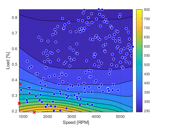
You want to operate the engine efficiently, so create a contour plot to see the region where the BSFC is low. Use the plot function, and specify the name/value parameter pair 'style','Contour'.
plot( f2, [Speed, Load], minBSFC, 'Exclude', out, 'Style', 'Contour' );
xlabel( 'Speed [RPM]' );
ylabel( 'Load [%]' );
colorbar
Create a Table from the Surface
Generate a table by evaluating the model f2 over a grid of points.
Create variables for the table breakpoints.
speedbreakpoints = linspace( 1000, 5500, 17 );
loadbreakpoints =  linspace( 0.2, 0.8, 13 );
To generate values for the table, evaluate the model over a grid of points.
[tSpeed, tLoad] = meshgrid( speedbreakpoints, loadbreakpoints );
tBSFC = f2( tSpeed, tLoad );
Examine the rows and columns of the table at the command line.
tBSFC(1:2:end,1:2:end)
ans =

  Columns 1 through 7

  722.3280  766.7608  779.4296  757.4574  694.5378  624.4095  576.5235
  503.9880  499.9201  481.7240  458.2803  427.7338  422.1099  412.1624
  394.7579  364.3421  336.1811  330.1550  329.1635  328.1810  329.1144
  333.7740  307.7736  295.1777  291.2068  290.3637  290.0173  287.8672
  295.9729  282.7567  273.8287  270.8869  269.8485  271.0547  270.5502
  273.7512  264.5167  259.7631  257.9215  256.9350  258.3228  258.6638
  251.5652  247.6746  247.2747  247.4699  247.3570  248.2433  248.8139

  Columns 8 through 9

  532.1533  466.9610
  396.3209  398.0199
  335.3871  346.3882
  286.3077  291.0075
  269.6837  272.2054
  258.0298  260.5269
  249.0083  250.4165
Plot the Table Against the Original Model
The grid on the model surface shows the table breakpoints.
h = plot( f2 );
h.EdgeColor = 'none';
hold on
mesh( tSpeed, tLoad, tBSFC, ...
    'LineStyle', '-', 'LineWidth', 2, 'EdgeColor', 'k', ...
    'FaceColor', 'none', 'FaceAlpha', 1 );
hold off
xlabel( 'Speed [RPM]' );
ylabel( 'Load [%]' );
zlabel( 'Minimum BSFC [g/Kwh]' );
Check the Table Accuracy
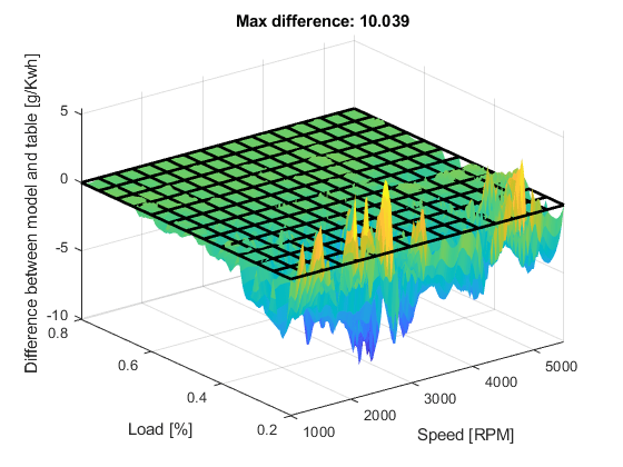
View the difference between the model and the table by plotting the difference between them on a finer grid. Then, use this difference in prediction accuracy between the table and the model to determine the most efficient table size for your accuracy requirements.
The following code evaluates the model over a finer grid and plots the difference between the model and the table.
[tfSpeed, tfLoad] = meshgrid( ...
    linspace( 1000, 5500, 8*17+1 ), ...
    linspace( 0.2, 0.8, 8*13+1 ) );
tfBSFC_model = f2( tfSpeed, tfLoad );
tfBSFC_table = interp2( tSpeed, tLoad, tBSFC, tfSpeed, tfLoad, 'linear' );
tfDiff = tfBSFC_model - tfBSFC_table;

surf( tfSpeed, tfLoad, tfDiff, 'LineStyle', 'none'  );
hold on
mesh( tSpeed, tLoad, zeros( size( tBSFC ) ), ...
    'LineStyle', '-', 'LineWidth', 2, 'EdgeColor', 'k', ...
    'FaceColor', 'none', 'FaceAlpha', 1 );
hold off
axis tight
xlabel( 'Speed [RPM]' );
ylabel( 'Load [%]' );
zlabel( 'Difference between model and table [g/Kwh]' );
title( sprintf( 'Max difference: %g', max( abs( tfDiff(:) ) ) ) );
Create a Table Array Including Breakpoint Values
After creating a table by evaluating a model fit over a grid of points, it can be useful to export your table data from MATLAB. Before exporting, create a table array that includes the breakpoint values in the first row and column. The following command reshapes your data to this table format:
X (
speedbreakpoints) is a (1 x M) vectorY (
loadbreakpoints) is an (N x 1) vectorZ (
tBSFC) is an (M x N) matrix
table = [
    {'Load\Speed'}, num2cell(speedbreakpoints(:).' )
    num2cell(loadbreakpoints (:) ), num2cell( tBSFC )
    ];
Export Table to Spreadsheet File
You can use the xlswrite function to export your table data to a new Excel Spreadsheet. Execute the following command to create a spreadsheet file.
xlswrite( 'tabledata.xlsx', table )
Create a Lookup Table Block
If you have Simulink® software, you can create a Look Up Table block as follows. Execute the following code to try it out.
1. Create a model with a 2-D Lookup Table block.
simulink
new_system( 'my_model' )
open_system( 'my_model' )
add_block( 'simulink/Lookup Tables/2-D Lookup Table', 'my_model/surfaceblock' )
2. Populate the Lookup Table with speed breakpoints, load breakpoints, and a lookup table.
set_param( 'my_model/surfaceblock',...
    'BreakpointsForDimension1', 'loadbreakpoints',...
    'BreakpointsForDimension2', 'speedbreakpoints',...
    'Table', 'tBSFC' );
3. Examine the populated Lookup Table block.
