Differentiating and Integrating a Fit
This example shows how to find the first and second derivatives of a fit, and the integral of the fit, at the predictor values.
Create a baseline sinusoidal signal:
xdata = (0:.1:2*pi)';
y0 = sin(xdata);
Add noise to the signal:
noise = 2*y0.*randn(size(y0)); % Response-dependent noise
ydata = y0 + noise;
Fit the noisy data with a custom sinusoidal model:
f = fittype('a*sin(b*x)');
fit1 = fit(xdata,ydata,f,'StartPoint',[1 1]);
Find the derivatives of the fit at the predictors:
[d1,d2] = differentiate(fit1,xdata);
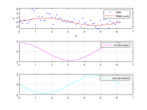
Plot the data, the fit, and the derivatives:
subplot(3,1,1)
plot(fit1,xdata,ydata) % cfit plot method
subplot(3,1,2)
plot(xdata,d1,'m') % double plot method
grid on
legend('1st derivative')
subplot(3,1,3)
plot(xdata,d2,'c') % double plot method
grid on
legend('2nd derivative')

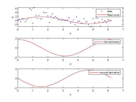
Note that derivatives can also be computed and plotted directly with the cfit plot method, as follows. The plot method, however, does not return data on the derivatives.
plot(fit1,xdata,ydata,{'fit','deriv1','deriv2'})

Find the integral of the fit at the predictors:
int = integrate(fit1,xdata,0);
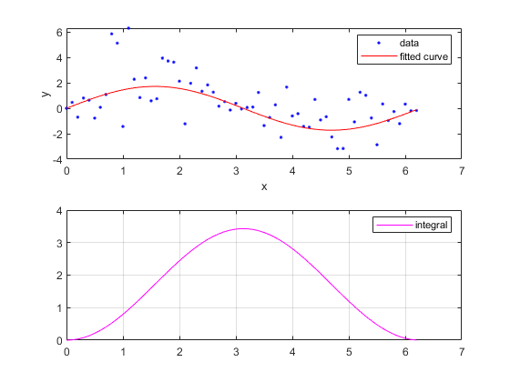
Plot the data, the fit, and the integral:
subplot(2,1,1)
plot(fit1,xdata,ydata) % cfit plot method
subplot(2,1,2)
plot(xdata,int,'m') % double plot method
grid on
legend('integral')

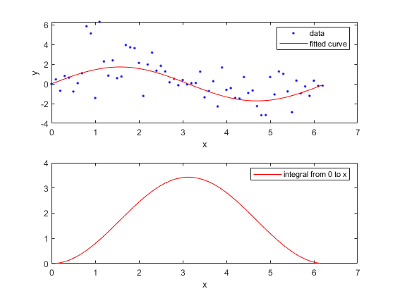
Note that integrals can also be computed and plotted directly with the cfit plot method, as follows. The plot method, however, does not return data on the integral.
plot(fit1,xdata,ydata,{'fit','integral'})

