bat365 Homepage

Approximation by Tensor Product Splines

Because the toolbox can handle splines with vector coefficients, it is easy to implement interpolation or approximation to gridded data by tensor product splines, as the following illustration is meant to show. You can also run the example “Bivariate Tensor Product Splines”.

To be sure, most tensor product spline approximation to gridded data can be obtained directly with one of the spline construction commands, like spapi or csape, in this toolbox, without concern for the details discussed in this example. Rather, this example is meant to illustrate the theory behind the tensor product construction, and this will be of help in situations not covered by the construction commands in this toolbox.

This section discusses these aspects of the tensor product spline problem:

Choice of Sites and Knots

Consider, for example, least squares approximation to given data z(i,j)=f(x(i),y(j)),i=1:Nx,j=1:Ny. You take the data from a function used extensively by Franke for the testing of schemes for surface fitting (see R. Franke, “A critical comparison of some methods for interpolation of scattered data,” Naval Postgraduate School Techn. Rep. NPS-53-79-003, March 1979). Its domain is the unit square. You choose a few more data sites in the x-direction than the y-direction; also, for a better definition, you use higher data density near the boundary.

x = sort([(0:10)/10,.03 .07, .93 .97]);
y = sort([(0:6)/6,.03 .07, .93 .97]);
[xx,yy] = ndgrid(x,y); z = franke(xx,yy);

Least Squares Approximation as Function of y

Treat these data as coming from a vector-valued function, namely, the function of y whose value at y(j) is the vector z(:,j), all j. For no particular reason, choose to approximate this function by a vector-valued parabolic spline, with three uniformly spaced interior knots. This means that you choose the spline order and the knot sequence for this vector-valued spline as

ky = 3; knotsy = augknt([0,.25,.5,.75,1],ky);

and then use spap2 to provide the least squares approximant to the data:

sp = spap2(knotsy,ky,y,z);

In effect, you are finding simultaneously the discrete least squares approximation from S_ky,knotsy to each of the Nx data sets

$\begin{matrix} {(y (j), z (i, j))}_{j = 1}^{N y}, & i = 1 : N x \end{matrix}$

In particular, the statements

yy = -.1:.05:1.1;
vals = fnval(sp,yy);

provide the array vals, whose entry vals(i,j) can be taken as an approximation to the value f(x(i),yy(j))of the underlying function f at the mesh-point x(i),yy(j) because vals(:,j) is the value at yy(j) of the approximating spline curve in sp.

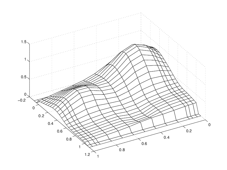
This is evident in the following figure, obtained by the command:

mesh(x,yy,vals.'), view(150,50)

Note the use of vals.', in the mesh command, needed because of the MATLAB^® matrix-oriented view when plotting an array. This can be a serious problem in bivariate approximation because there it is customary to think of z(i, j) as the function value at the point (x(i), y(j)), while MATLAB thinks of z(i, j) as the function value at the point (x(j), y(i)).

A Family of Smooth Curves Pretending to Be a Surface

Note that both the first two and the last two values on each smooth curve are actually zero because both the first two and the last two sites in yy are outside the basic interval for the spline in sp.

Note also the ridges. They confirm that you are plotting smooth curves in one direction only.

Approximation to Coefficients as Functions of x

To get an actual surface, you now have to go a step further. Look at the coefficients coefsy of the spline in sp:

coefsy = fnbrk(sp,'coefs');

Abstractly, you can think of the spline in sp as the function

$y | \to \sum_{r} c o e f s y (:, r) B_{r, k y} (y)$

with the ith entry coefsy(i,r) of the vector coefficient coefsy(:,r) corresponding to x(i), for all i. This suggests approximating each coefficient vector coefsy(q,:) by a spline of the same order kx and with the same appropriate knot sequence knotsx. For no particular reason, this time use cubic splines with four uniformly spaced interior knots:

kx = 4; knotsx = augknt([0:.2:1],kx); 
sp2 = spap2(knotsx,kx,x,coefsy.');

Note that spap2(knots,k,x,fx) expects fx(:,j) to be the datum at x(j), i.e., expects each column of fx to be a function value. To fit the datum coefsy(q, :) at x(q), for all q, present spap2 with the transpose of coefsy.

The Bivariate Approximation

Now consider the transpose of the coefficients cxy of the resulting spline curve:

coefs = fnbrk(sp2,'coefs').';

It provides the bivariate spline approximation

$(x, y) | \to \sum_{q} \sum_{r} c o e f s (q, r) B_{q, k x} (x) B_{r, k y} (y)$

to the original data

$(x (i), y (j)) | \to z (x (i), y (j)), i = 1 : N x, j = 1 : N y$

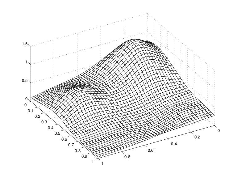
To plot this spline surface over a grid, e.g., the grid

xv = 0:.025:1; yv = 0:.025:1;

you can do the following:

values = spcol(knotsx,kx,xv)*coefs*spcol(knotsy,ky,yv).'; 
mesh(xv,yv,values.'), view(150,50);

This results in the following figure.

Spline Approximation to Franke's Function

This makes good sense because spcol(knotsx,kx,xv) is the matrix whose (i,q)th entry equals the value B_q,kx(xv(i)) at xv(i) of the qth B-spline of order kx for the knot sequence knotsx.

Because the matrices spcol(knotsx,kx,xv) and spcol(knotsy,ky,yv) are banded, it may be more efficient, though perhaps more memory-consuming, for large xv and yv to make use of fnval, as follows:

value2 = ... 
  fnval(spmak(knotsx,fnval(spmak(knotsy,coefs),yv).'),xv).';

This is, in fact, what happens internally when fnval is called directly with a tensor product spline, as in

value2 = fnval(spmak({knotsx,knotsy},coefs),{xv,yv});

Here is the calculation of the relative error, i.e., the difference between the given data and the value of the approximation at those data sites as compared with the magnitude of the given data:

errors = z - spcol(knotsx,kx,x)*coefs*spcol(knotsy,ky,y).'; 
disp( max(max(abs(errors)))/max(max(abs(z))) )

The output is 0.0539, perhaps not too impressive. However, the coefficient array was only of size 8 6

disp(size(coefs))

to fit a data array of size 15 11.

disp(size(z))

Switch in Order

The approach followed here seems biased, in the following way. First think of the given data z as describing a vector-valued function of y, and then treat the matrix formed by the vector coefficients of the approximating curve as describing a vector-valued function of x.

What happens when you take things in the opposite order, i.e., think of z as describing a vector-valued function of x, and then treat the matrix made up from the vector coefficients of the approximating curve as describing a vector-valued function of y?

Perhaps surprisingly, the final approximation is the same, up to round-off. Here is the numerical experiment.

Least Squares Approximation as Function of x

First, fit a spline curve to the data, but this time with x as the independent variable, hence it is the rows of z that now become the data values. Correspondingly, you must supply z.', rather than z, to spap2,

spb = spap2(knotsx,kx,x,z.');

thus obtaining a spline approximation to all the curves (x ; z (:, j)). In particular, the statement

valsb = fnval(spb,xv).';

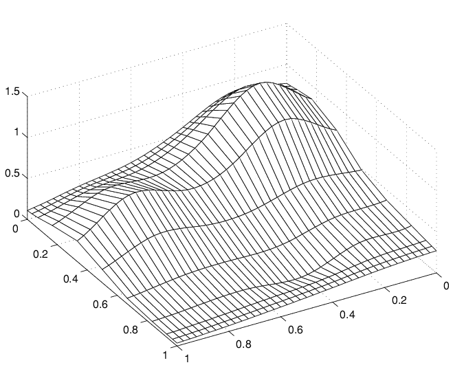
provides the matrix valsb, whose entry valsb(i, j) can be taken as an approximation to the value f(xv(i),y(j)) of the underlying function f at the mesh-point (xv(i),y(j)). This is evident when you plot valsb using mesh:

mesh(xv,y,valsb.'), view(150,50)

Another Family of Smooth Curves Pretending to Be a Surface

Note the ridges. They confirm that you are, once again, plotting smooth curves in one direction only. But this time the curves run in the other direction.

Approximation to Coefficients as Functions of y

Now comes the second step, to get the actual surface. First, extract the coefficients:

coefsx = fnbrk(spb,'coefs');

Then fit each coefficient vector coefsx(r,:) by a spline of the same order ky and with the same appropriate knot sequence knotsy:

spb2 = spap2(knotsy,ky,y,coefsx.');

Note that, once again, you need to transpose the coefficient array from spb, because spap2 takes the columns of its last input argument as the data values.

Correspondingly, there is now no need to transpose the coefficient array coefsb of the resulting curve:

coefsb = fnbrk(spb2,'coefs');

The Bivariate Approximation

The claim is that coefsb equals the earlier coefficient array coefs, up to round-off, and here is the test:

disp( max(max(abs(coefs - coefsb))) )

The output is 1.4433e-15.

The explanation is simple enough: The coefficients c of the spline s contained in sp = spap2(knots,k,x,y) depend linearly on the input values y. This implies, given that both c and y are 1-row matrices, that there is some matrix A=A_knots,k,x so that

$c = y A_{knots, k, x}$

for any data y. This statement even holds when y is a matrix, of size d-by-N, say, in which case each datum y(:,j) is taken to be a point in R^d, and the resulting spline is correspondingly d-vector-valued, hence its coefficient array c is of size d-by-n, with n = length(knots)-k.

In particular, the statements

sp = spap2(knotsy,ky,y,z); 
coefsy =fnbrk(sp,'coefs');

provide us with the matrix coefsy that satisfies

$coefs y = z . A_{knotsy,ky,y}$

The subsequent computations

 sp2 = spap2(knotsx,kx,x,coefsy.'); 
 coefs = fnbrk(sp2,'coefs').';

generate the coefficient array coefs, which, taking into account the two transpositions, satisfies

$\begin{matrix} coefs = ((z A_{knotsy,ky,y})' . A_{knotsx,kx,x})' \\ = (A_{knotsx,kx,x})' . z . A_{knotsy,ky,y} \end{matrix}$

In the second, alternative, calculation, you first computed

 spb = spap2(knotsx,kx,x,z.'); 
 coefsx = fnbrk(spb,'coefs');

hence coefsx=z'.A_knotsx,kx,x. The subsequent calculation

 spb2 = spap2(knotsy,ky,y,coefsx.');
 coefsb = fnbrk(spb,'coefs');

then provided

$coefsb = coefsx .' . A_{knotsy,ky,y} = (A_{knotsx,kx,x}) .' . z . A_{knotsy,ky, y}$

Consequently, coefsb = coefs.

Comparison and Extension

The second approach is more symmetric than the first in that transposition takes place in each call to spap2 and nowhere else. This approach can be used for approximation to gridded data in any number of variables.

If, for example, the given data over a three-dimensional grid are contained in some three-dimensional array v of size [Nx,Ny,Nz], with v(i,j,k) containing the value f(x(i),y(j),z(k)), then you would start off with

coefs = reshape(v,Nx,Ny*Nz);

Assuming that nj = knotsj - kj, for j = x,y,z, you would then proceed as follows:

sp = spap2(knotsx,kx,x,coefs.');
coefs = reshape(fnbrk(sp,'coefs'),Ny,Nz*nx);
sp = spap2(knotsy,ky,y,coefs.'); 
coefs = reshape(fnbrk(sp,'coefs'),Nz,nx*ny);
sp = spap2(knotsz,kz,z,coefs.'); 
coefs = reshape(fnbrk(sp,'coefs'),nx,ny*nz);

See Chapter 17 of PGS or [C. de Boor, “Efficient computer manipulation of tensor products,” ACM Trans. Math. Software 5 (1979), 173–182; Corrigenda, 525] for more details. The same references also make clear that there is nothing special here about using least squares approximation. Any approximation process, including spline interpolation, whose resulting approximation has coefficients that depend linearly on the given data, can be extended in the same way to a multivariate approximation process to gridded data.

This is exactly what is used in the spline construction commands csapi, csape, spapi, spaps, and spap2, when gridded data are to be fitted. It is also used in fnval, when a tensor product spline is to be evaluated on a grid.