Learn optimal hyperplanes as decision boundaries
A support vector machine (SVM) is a supervised learning algorithm used for many classification and regression problems, including signal processing medical applications, natural language processing, and speech and image recognition.
The objective of the SVM algorithm is to find a hyperplane that, to the best degree possible, separates data points of one class from those of another class. “Best” is defined as the hyperplane with the largest margin between the two classes, represented by plus versus minus in the figure below. Margin means the maximal width of the slab parallel to the hyperplane that has no interior data points. Only for linearly separable problems can the algorithm find such a hyperplane, for most practical problems the algorithm maximizes the soft margin allowing a small number of misclassifications.

Defining the “margin” between classes – the criterion that SVMs seek to optimize.
Support vectors refer to a subset of the training observations that identify the location of the separating hyperplane. The standard SVM algorithm is formulated for binary classification problems, and multiclass problems are typically reduced to a series of binary ones.
Digging deeper into the mathematical details, support vector machines fall under a class of machine learning algorithms called kernel methods where the features can be transformed using a kernel function. Kernel functions map the data to a different, often higher dimensional space with the expectation that the classes are easier to separate after this transformation, potentially simplifying a complex non-linear decision boundaries to linear ones in the higher dimensional, mapped feature space. In this process, the data doesn’t have to be explicitly transformed, which would be computationally expensive. This is commonly known as the kernel trick.
MATLAB® supports several kernels including:
| Type of SVM | Mercer Kernel | Description |
|---|---|---|
| Gaussian or Radial Basis Function (RBF) | \(K(x_1,x_2) = \exp\left(-\frac{\|x_1 - x_2\|^2}{2\sigma^2}\right)\) | One class learning. \(\sigma\)is the width of the kernel |
| Linear | \(K(x_1,x_2) = x_1^{\mathsf{T}}x_2\) |
Two class learning. |
| Polynomial | \(K(x_1,x_2) = \left( x_1^{\mathsf{T}}x_2 + 1 \right)^{\rho}\) |
\(\rho\) is the order of the polynomial |
| Sigmoid | \(K(x_1,x_2) = \tanh\left( \beta_{0}x_1^{\mathsf{T}}x_2 + \beta_{1} \right)\) |
It is a mercer kernel for certain \(\beta_{0}\) and \(\beta_{1}\) values only |
Training a support vector machine corresponds to solving a quadratic optimization problem to fit a hyperplane that minimizes the soft margin between the classes. The number of transformed features is determined by the number of support vectors.
Key points:
- Support vector machines are popular and achieve good performance on many classification and regression tasks.
- While support vector machines are formulated for binary classification, you construct a multi-class SVM by combining multiple binary classifiers.
- Kernels make SVMs more flexible and able to handle nonlinear problems.
- Only the support vectors chosen from the training data are required to construct the decision surface. Once trained, the rest of the training data is irrelevant, yielding a compact representation of the model that is suitable for automated code generation.
Example
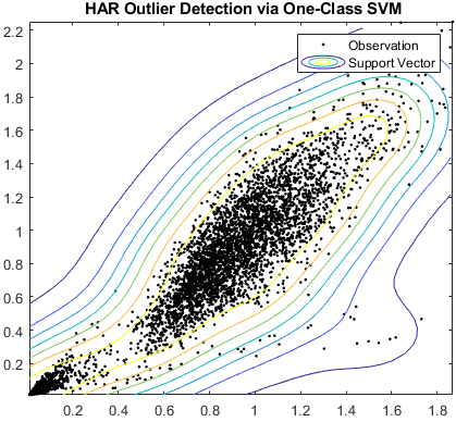
Support vector machines can also be used for anomaly detection by constructing a one-class SVM whose decision boundary determines whether an object belongs to the “normal” class using an outlier threshold. In this example, MATLAB maps all examples to a single class based on the targeted fraction of outliers as parameter as follows: fitcsvm(sample,ones(…), ‘OutlierFraction’, …). The graph shows the separating hyperplanes for a range of OutlierFractions for data from a human activity classification task.

Examples and How To
Software Reference
See also: Statistics and Machine Learning Toolbox, machine learning with MATLAB, Machine Learning Models, biomedical signal processing
